1. Intro to ML & Decision Trees#

1.1. Welcome#

Welcome to Bait 509 - Business Application of Machine Learning!

Note

Buckle up because there are going to be a lot of new concepts here but in the lyrics of Trooper “We’re here for a good time, Not a long time”.

1.1.1. Course Learning Objectives#

Describe fundamental machine learning concepts such as: supervised and unsupervised learning, regression and classification, overfitting, training/validation/testing error, parameters and hyperparameters, and the golden rule.
Broadly explain how common machine learning algorithms work, including: naïve Bayes, k-nearest neighbors, decision trees, support vector machines, and logistic regression.
Identify when and why to apply data pre-processing techniques such as scaling and one-hot encoding.
Use Python and the scikit-learn package to develop an end-to-end supervised machine learning pipeline.
Apply and interpret machine learning methods to carry out supervised learning projects and to answer business objectives.

1.1.2. Python, Jupyter, Visualizations#

In this course we be using Python and Jupyter notebooks for lectures as well as assignments.
I recommend using the Miniconda distribution to install and manage your Python package installations, but you are free to use either Anaconda or pip if you prefer that.
If you are using Miniconda or Anaconda, you can install a few key packages we will be using in the course, by typing the following at the command line (the “Anaconda prompt” on Windows, and the default terminal application on MacOS/Linux):

conda install xgboost jupyter altair_saver seaborn
Otherwise you can use pip and type the following at the command line:

pip install xgboost jupyter altair_saver seaborn
Some packages that we will make heavy use of are installed together with the packages above, most notably pandas, numpy, matplotlib, and scikit-learn.

We will be making visualizations for this course and I give the option of plotting using any Python library (e.g. matplotlib, seaborn, pandas, altair, etc.) but I strongly recommend getting familiar with altair. I have 2 very quick slide decks that teach you a bit about how to plot using altair. From the course Programming in Python for Data Science
- Module 1, exercise 31, 32, 33
- Module 2, exercise 29, 30
- And if you want to dive further there is a whole course dedicated to visualizing plots using altair called Data Visualization.

1.1.3. Lecture Learning Objectives#

Don’t worry if some of these terms don’t make sense up front, they will after we have covered them during today’s lecture.

Explain motivation to study machine learning.
Differentiate between supervised and unsupervised learning.
Differentiate between classification and regression problems.
Explain machine learning terminology such as features, targets, training, and error.
Explain the .fit() and .predict() paradigm and use .score() method of ML models.
Broadly describe how decision trees make predictions.
Use DecisionTreeClassifier() and DecisionTreeRegressor() to build decision trees using scikit-learn.
Explain the difference between parameters and hyperparameters.
Explain how decision boundaries change with max_depth.

1.2. What is Machine Learning (ML)?#

Machine learning is all around us. You can find it in things like:

Voice assistance
Google news
Recommender systems
Face recognition
Auto completion
Stock market predictions
Character recognition
Self-driving cars
Cancer diagnosis
Drug discovery

Machine Learning can mean many different things to different people. In this course, we will stick to how it is defined in the seminal textbook “Introduction to Statistical Learning” which defines Statistical/Machine Learning as a “set of tools for making sense of complex datasets”. As you can hear, this is still rather broad, and we will refine our understanding throughout this course. Let’s start right now by looking at some specific examples of Machine Learning problems.

1.3. Types of Machine Learning#

Supervised learning (this course)
Unsupervised learning

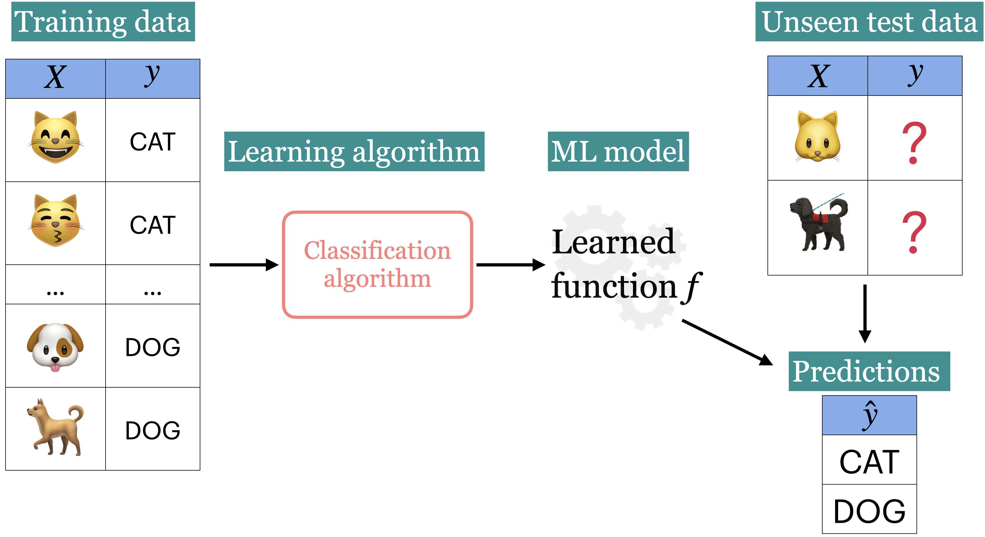
1.3.1. Supervised Learning:#

Example: Labelling emails as spam or not

In supervised machine learning, we have a set of observations usually denoted with an uppercase X.
We also have a set of corresponding targets usually denoted with a lowercase y.
Our goal is to define a function that relates X to y.
We then use this function to predict the targets of new examples.

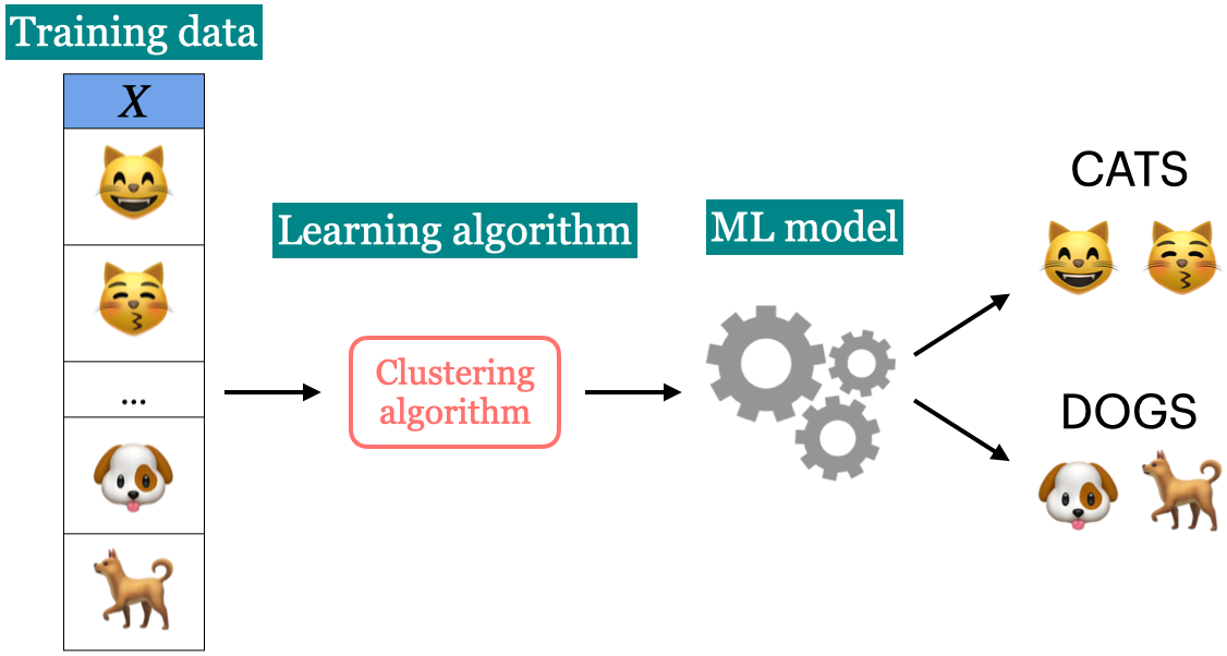
1.3.2. UnSupervised Learning: (not going into detail here)#

Example: Categorizing Google News articles.

In unsupervised learning, we are not given target labels and are instead only given observations X.
We apply an algorithm to try find patterns/structure in our data and divide the observations into groups/clusters that share similar characteristics from our data.
E.g. it could be that we want find out if there are groups of business that operate similarly based a few key business metrics. We might not know up front how many groups there are in the data, and an unsupervised clustering algorithm could help us understand if there e.g. are two very distinct set of strategies that business employ (two clusters), or if there is a big mix and no clear structure at all in our data.
Another example can be seen below, we might get input images of cats and dogs and ask the algorithm to cluster them together based on any property that can be extracted from the images (color, size, shapes, etc).

1.4. Types of Supervised Learning: Classification vs Regression#

Classification
Regression

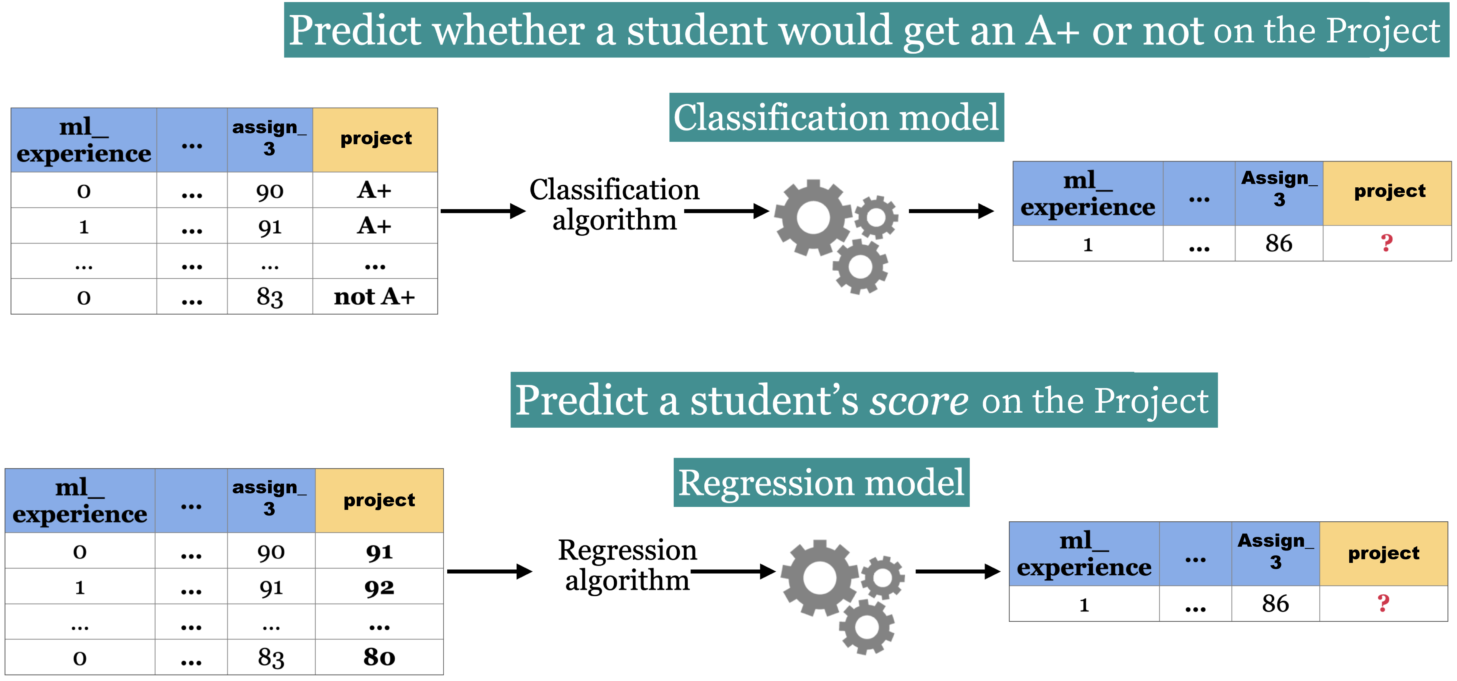
1.4.1. Classification#

Classification predicting among two or more categories, also known as classes.

Example1: Predict whether a customer will default on their credit card or not.
Example2: Predict whether a student would get an A+ or not in a project.

1.4.2. Regression#

Regression predicting a continuous (in other words, a number) value.

Example1: Predict housing prices
Example2: Predict a student’s score in a project.

Example 1: Credit card fraud detection data set

In this example, we are trying to predict whether a person is likely to default (class = 1) or not (class = 0) on their credit card given a bunch of input features.

import pandas as pd

classification_df = pd.read_csv("data/creditcard_sample.csv").sample(10_000, random_state=390)
classification_df.head(5)

Example 2: Predict housing sale price

In this example, we are trying to predict the sale price of a house given its features such as number of bedroom, number of bathrooms, sqft, etc.

regression_df = pd.read_csv("data/kc_house_data.csv").drop(columns=["id", "date"])
regression_df.head(5)

1.5. Let’s Practice#

Are the following supervised or unsupervised problems?

1. Finding groups of similar properties in a real estate data set.
2. Predicting real estate prices based on house features like number of rooms, learning from past sales as examples.
3. Identifying groups of animals given features such as “number of legs”, “wings/no wings”, “fur/no fur”, etc.
4. Detecting heart disease in patients based on different test results and history.
5. Grouping articles on different topics from different news sources (something like Google News app).

Are the following classification or regression problems?

6. Predicting the price of a house based on features such as number of rooms and the year built.
7. Predicting if a house will sell or not based on features like the price of the house, number of rooms, etc.
8. Predicting your grade in BAIT 509 based on past grades.
9. Predicting whether you should bicycle tomorrow or not based on the weather forecast.
10. Predicting a cereal’s manufacturer given the nutritional information.

Solutions!

Unsupervised
Supervised
Unsupervised
Supervised
Unsupervised
Regression
Classification
Regression
Classification
Classification

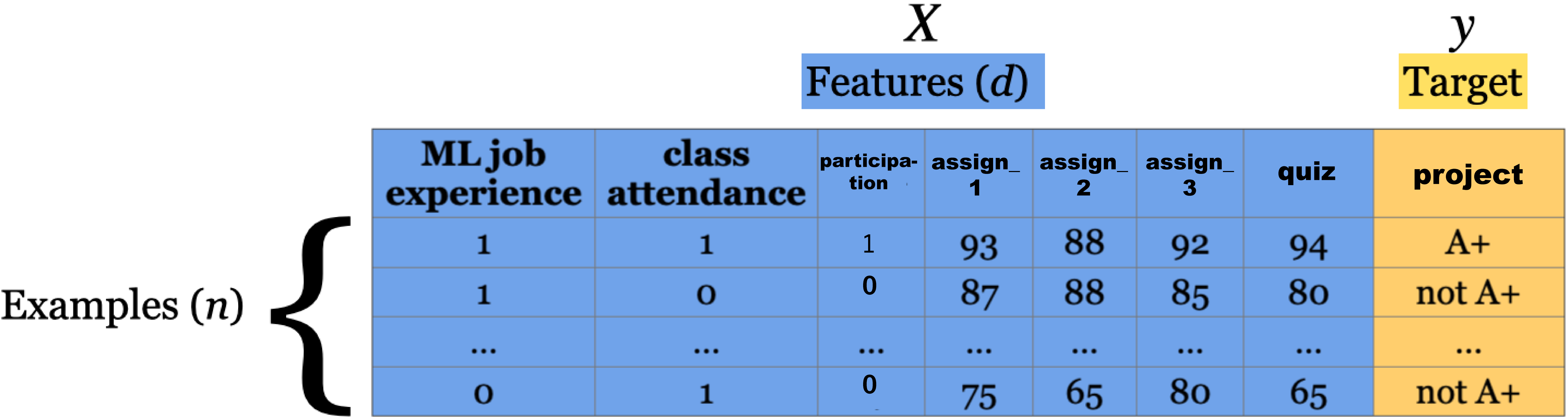
1.6. Tabular Data and Terminology#

Basic terminology used in ML:

examples/observations = rows
features/variables = inputs (columns)
targets = outputs (one special column)
training = learning = fitting

1.6.1. Example:#

This dataset contains longtitude and latitude data for 400 cities in the US.
Each city is labelled as red or blue depending on how they voted in the 2012 election.

df = pd.read_csv('data/cities_USA.csv', index_col=0).sample(12, random_state=89)
df

df.shape

In this dataset, we have:

2 features, (3 columns = 2 features + 1 target) and,
20 examples.

Our target column is vote since that is what we are interesting in predicting.

1.7. Decision Tree Algorithm#

1.7.1. A conceptual introduction to Decision Trees#

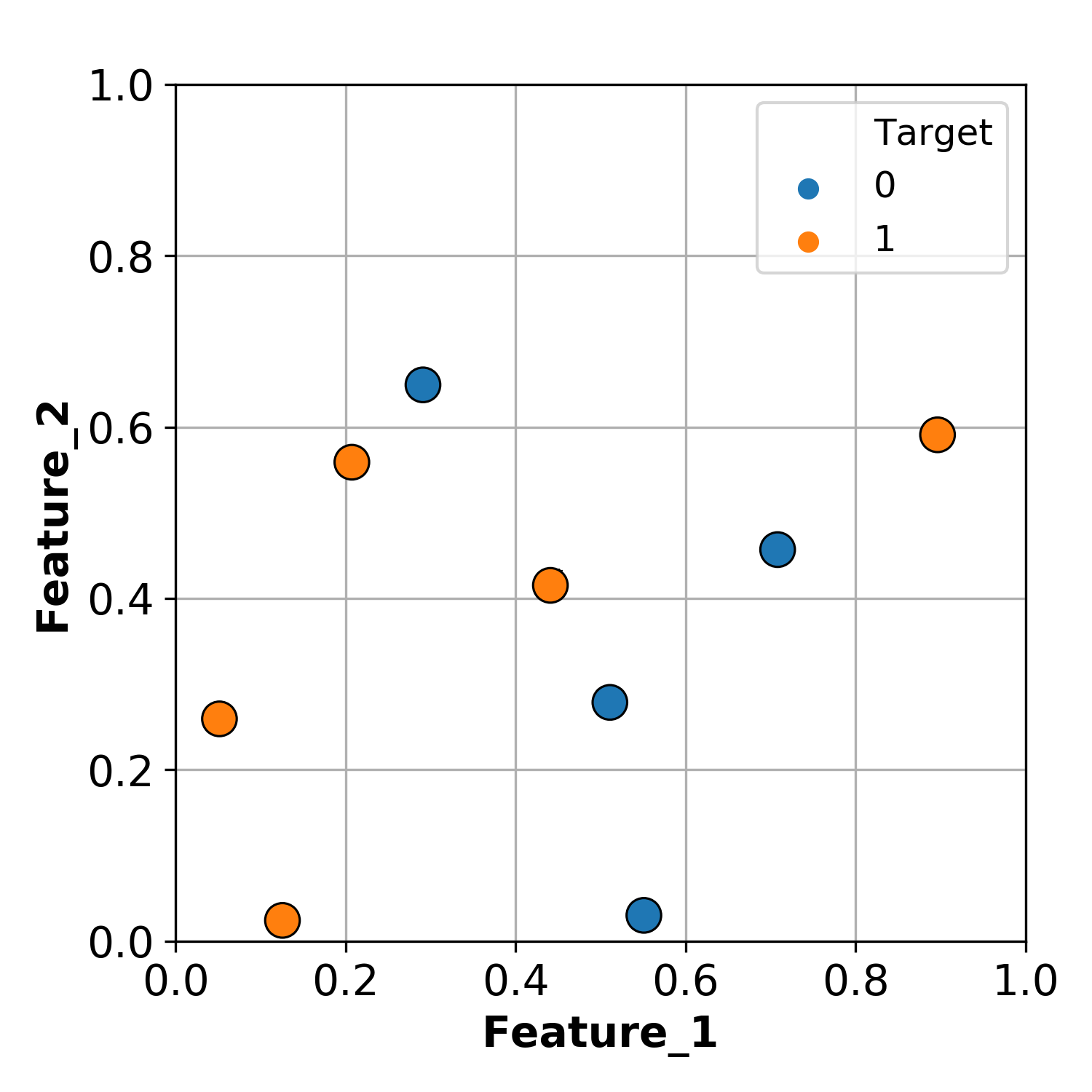
Shown below is some hypothetical data with 2 features (x and y axes) and 1 target (with 2 classes).
The supervised learning problem here is to predict whether a particular observaton belongs to the BLUE or ORANGE class.
A fairly intuitive way to do this is to simply use thresholds to split the data up.

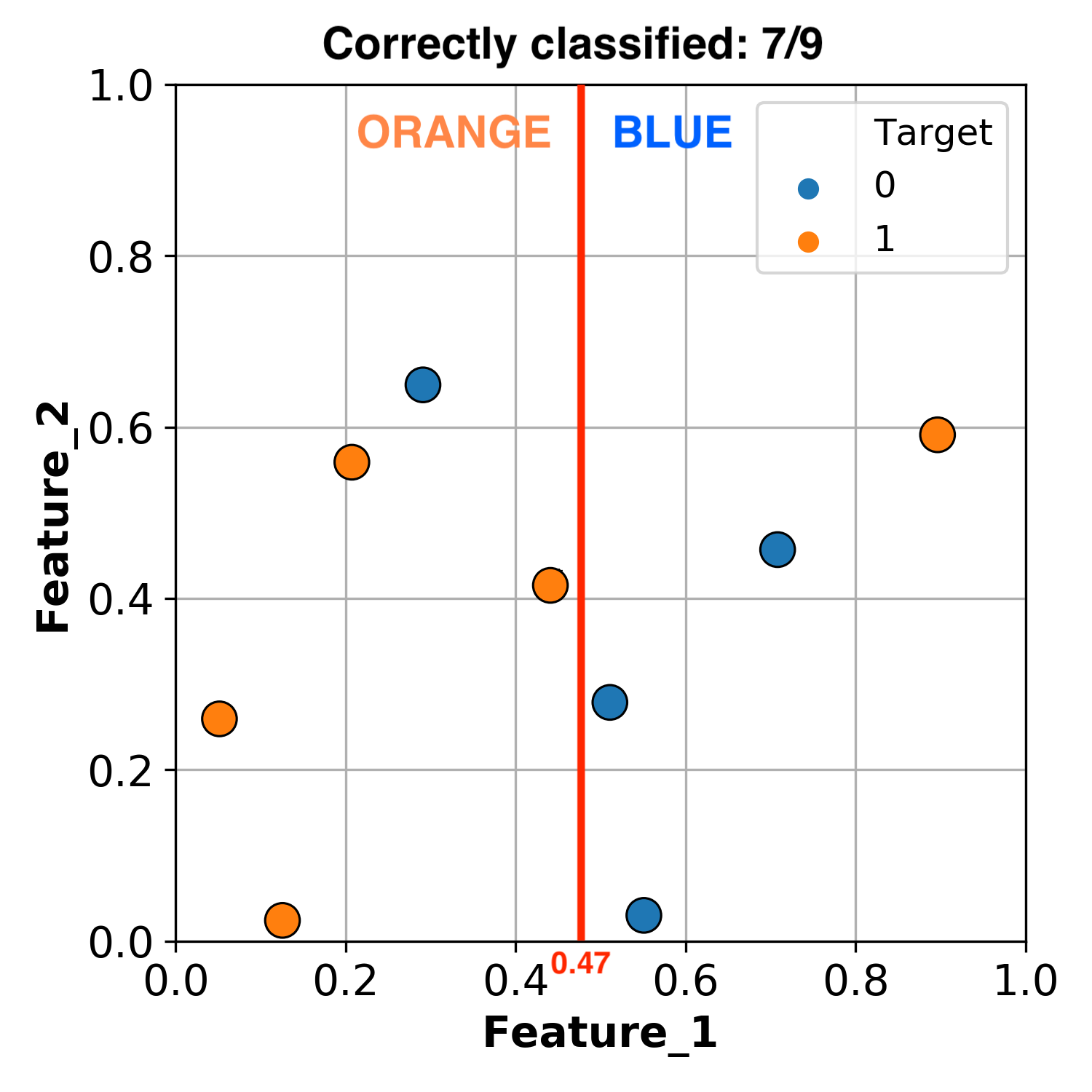
For example, we can split the data at Feature_1 = 0.47.
Everything less than the split we can classify as ORANGE.
Everything greater than the split we can classify as BLUE.
By this method, we can successfully classify 7 / 9 observations.

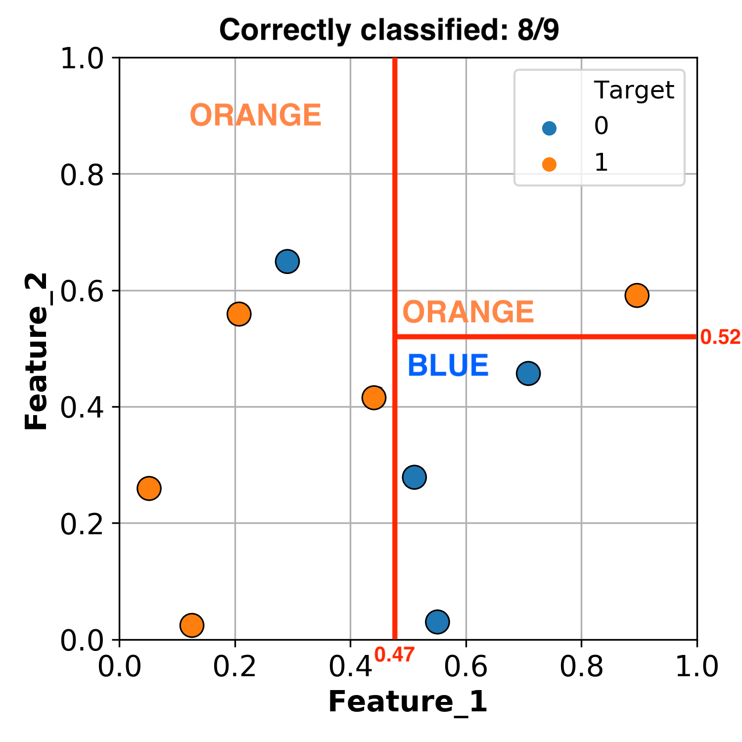
But we don’t have to stop there, we can make another split!
Let’s now split the section that is greater than Feature_1 = 0.47, using Feature_2 = 0.52. We now have the following conditions:

If Feature_1 > 0.47 and Feature_2 < 0.52 classify as BLUE.
If Feature_1 > 0.47 and Feature_2 > 0.52 classify as ORANGE.

Using these rules, we now successfully classify 8 / 9 observations.

Okay, let’s add one more threshhold.
Let’s make a final split of the section that is less than Feature_1 = 0.47, using Feature_2 = 0.6.
By this methodology we have successfully classified all of our data.

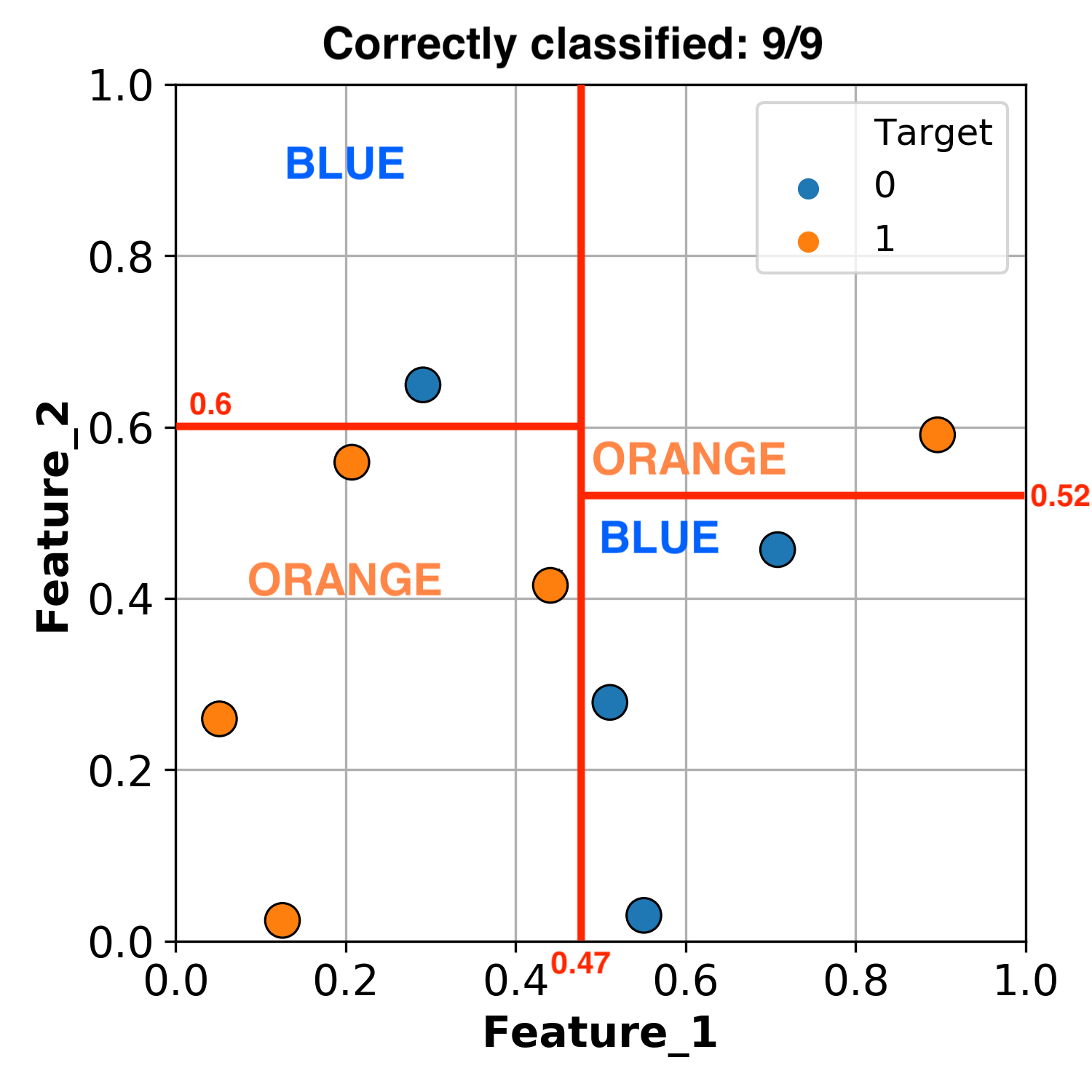
What we’ve really done here is create a group of if statements:

If Feature_1 < 0.47 and Feature_2 < 0.6 classify as ORANGE
If Feature_1 < 0.47 and Feature_2 > 0.6 classify as BLUE
If Feature_1 > 0.47 and Feature_2 < 0.52 classify as BLUE
If Feature_1 > 0.47 and Feature_2 > 0.52 classify as ORANGE

This is easier to visualize as a tree:

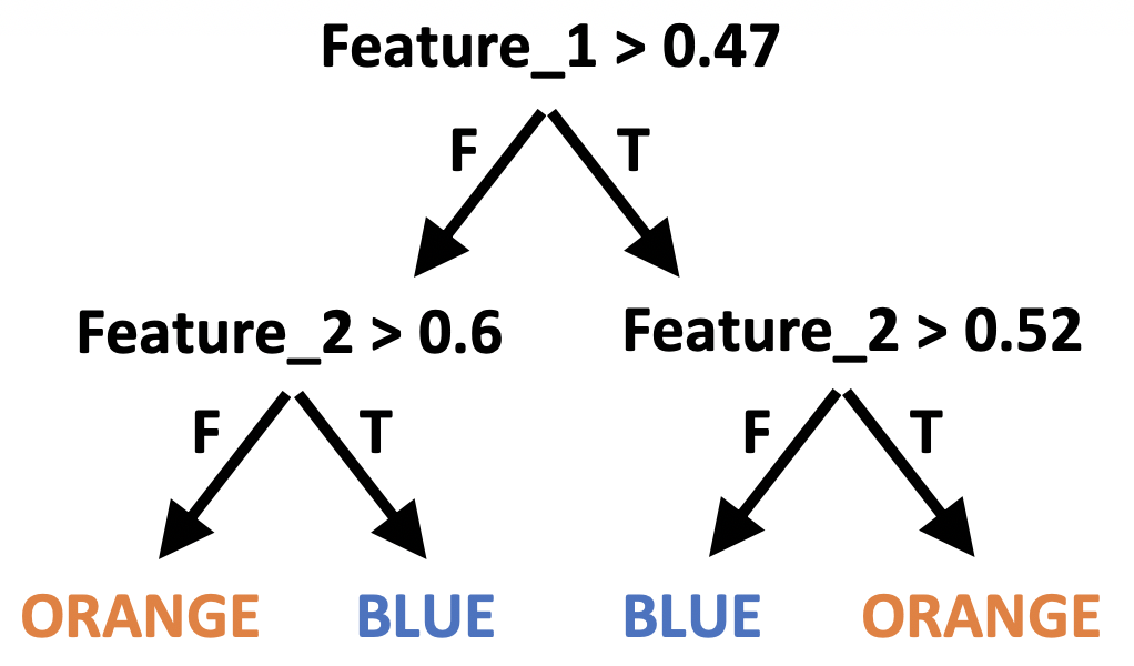
We just made our first decision tree!

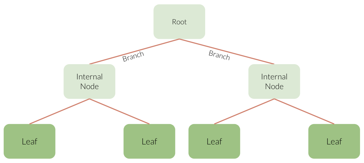
Before we go forward with learning about decision tree classifiers and reggressors we need to understand the structure of a decision tree. Here is the key terminology that you will have to know:

Root: Where we start making our conditions.
Branch: A branch connects to the next node (statement). Each branch represents either true or false.
Internal node: conditions within the tree.
Leaf: the value predicted from the conditions.
Tree depth: The longest path from the root to a leaf.

With the decision tree algorithm in machine learning, the tree can have at most two nodes resulting from it, also known as children.

If a tree only has a depth of 1, we call that a decision stump.

This tree and the one in our example above, both have a depth of 2.

Trees do not need to be balanced. (You’ll see this shortly)

1.7.2. Implimentation with Scikit-learn#

Steps to train a classifier using sklearn:

Read the data
Create $X$ and $y$
Create a classifier object
fit the classifier
predict on new examples
score the model

1.7.2.1. 1. Read the data#

df = pd.read_csv('data/cities_USA.csv', index_col=0).sample(40, random_state=89)
df.head()

	lon	lat	vote
146	-82.155358	38.008878	blue
33	-92.744478	31.226442	blue
389	-96.505225	47.070528	red
297	-87.964364	42.159843	red
230	-88.137965	40.374736	red

1.7.2.2. 2. Create $X$ and $y$#

Before we build any model (we are getting to that so hang tight), we need to make sure we have the right “parts” aka inputs and outputs.

That means we need to split up our tabular data into the features and the target, also known as $X$ and $y$.

$X$ is all of our features in our data, which we also call our feature table.
$y$ is our target, which is what we are predicting.

X = df.drop(columns=["vote"])
y = df["vote"]

X.head()

	lon	lat
146	-82.155358	38.008878
33	-92.744478	31.226442
389	-96.505225	47.070528
297	-87.964364	42.159843
230	-88.137965	40.374736

y.head()

  blue
   blue
   red
   red
   red
Name: vote, dtype: object

1.7.2.3. 3. Create a classifier object#

import the appropriate classifier
Create an object of the classifier

There are several machine learning libraries available to use but for this course, we will be using the Scikit-learn (hereafter, referred to as sklearn) library, which is a popular (41.6k stars on Github) Machine Learning library for Python.

We generally import a particular ML algorithm using the following syntax:

from sklearn.module import algorithm

The decision tree classification algorithm (DecisionTreeClassifier) sits within the tree module.
(Note there is also a Decision Tree Regression algorithm in this module which we’ll come to later…)
Let’s import the classifier using the following code:

from sklearn.tree import DecisionTreeClassifier

We can begin creating a model by instantiating an instance of the algorithm class.
Here we are naming our decision tree model model:

model = DecisionTreeClassifier()
model

DecisionTreeClassifier()

In a Jupyter environment, please rerun this cell to show the HTML representation or trust the notebook.
On GitHub, the HTML representation is unable to render, please try loading this page with nbviewer.org.

# help(DecisionTreeClassifier)

At this point we just have the framework of a model.
We can’t do anything with our algorithm yet, because it hasn’t seen any data!
We need to give our algorithm some data to learn/train/fit a model.

1.7.2.4. 4. Fit the classifier#

We can now use the .fit() method to train our model using the feature X and target y data we just separated.
When we call fit on our model object, the actual learning happens.

model.fit(X, y)

DecisionTreeClassifier()

In a Jupyter environment, please rerun this cell to show the HTML representation or trust the notebook.
On GitHub, the HTML representation is unable to render, please try loading this page with nbviewer.org.

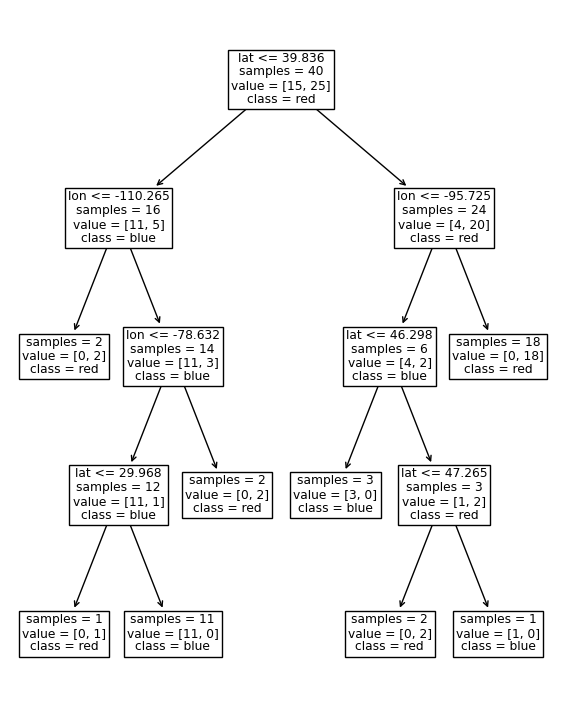
Now we’ve used data to learn a model, let’s take a look at the model we made!
The code below prints out our model structure for us (like the tree we made ourselves earlier)

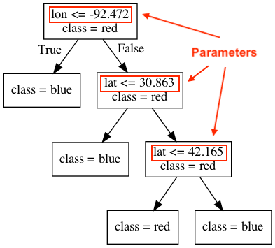
The way to read the decision tree visualization below is that if the condition on top of a box is true, then you follow the left arrow and if it is false you follow the right arrow. samples indicated how many observations there are in the node and values how many of those are [blue, red]. The class of each node indicated what class most samples in that node belong to. Note that you need to make sure that the feature and class names are passed in the correct order, and the best way to do this is to crosscheck with the next plot we will make, but for now you can rely on that I have put these in the expected order.

from sklearn.tree import plot_tree
import matplotlib.pyplot as plt


plot_tree(
    model,
    feature_names=X.columns,
    class_names=y.unique(),
    impurity=False,
    ax=plt.subplots(figsize=(7, 9))[1]  # We need to create a figure to control the overall plot size
);

We can better visualize what’s going on by actually plotting our data and the model’s decision boundaries.

# import a custom function

import os
import sys
sys.path.append(os.path.join(os.path.abspath("."), "code"))
from plotting_functions import *
from utils import *

plot_tree_decision_boundary_and_tree(
    model,
    X,
    y,
    height=6,
    width=16,
    fontsize=15,
    eps=10,
    x_label="lon",
    y_label="lat",
)

/Users/quannguyen/opt/miniconda3/envs/571/lib/python3.10/site-packages/sklearn/base.py:465: UserWarning: X does not have valid feature names, but DecisionTreeClassifier was fitted with feature names
  warnings.warn(

In this plot the shaded regions show what our model predicts for different feature values.
The scatter points are our actual 20 observations.
From the above plot, we can see that our model is classifying all our observations correctly, but there’s an easier way to find out how our model is doing.

How does .fit() work?

Or “How does do Decision Trees decide what values to split on?”

We will not go into detail here, but in general the algorithm is trying to maximize the homogeneity of the target variable within each of the groups created from a split. In other words, observations on the left of a split should all be similar to each other and observation on the right of the split should all be similar to each other.

There are different ways to measure similarity between observations and some of the most common metrics include:

Gini Index
Information gain
Cross entropy

You can read more about these metrics here

1.7.2.5. 5. Predict the target using unseen data#

We can predict the target of examples by calling .predict() on the classifier object.
Let’s see what it predicts for a single randomly new observation first:

new_ex = [-87.4, 59]
new_example = pd.DataFrame(data=[new_ex], columns=["lon", "lat"])
new_example

model.predict(new_example)

array(['red'], dtype=object)

we get a prediction of red for this example!

We can also predict on our whole feature table - Here, we are predicting on all of X.

model.predict(X)

pd.DataFrame({'true_values' : y.to_numpy(), 'predicted' : model.predict(X)})

	true_values	predicted
0	blue	blue
1	blue	blue
2	red	red
3	red	red
4	red	red
5	red	red
6	blue	blue
7	blue	blue
8	red	red
9	blue	blue
10	blue	blue
11	red	red
12	red	red
13	blue	blue
14	blue	blue
15	red	red
16	red	red
17	red	red
18	red	red
19	blue	blue
20	blue	blue
21	red	red
22	blue	blue
23	blue	blue
24	red	red
25	red	red
26	blue	blue
27	red	red
28	red	red
29	red	red
30	red	red
31	blue	blue
32	red	red
33	blue	blue
34	red	red
35	red	red
36	red	red
37	red	red
38	red	red
39	red	red

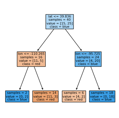
How does .predict() work?

For us to see how our algorithm predicts for each example, all we have to do is return to our Decision Tree.

plot_tree(
    model,
    feature_names=X.columns,
    class_names=y.unique(),
    impurity=False,
    ax=plt.subplots(figsize=(4, 5))[1]
);

Let’s use our new_example object for this example.

new_example

First we start at the root.
Is lat <= 39.727? False, so we go down the right branch.
Is lon <= -98.139? False , so we go down the right branch.
and arrive at red!

Let’s check this using predict again.

model.predict(new_example)

Nice!

1.7.2.6. 6. Score the model#

How do you know how well your model is doing?
For classification problems, by default, score gives the accuracy of the model, i.e., proportion of correctly predicted targets.

$accuracy = \frac{\text{correct predictions}}{\text{total examples}}$

print("The accuracy of the model on the training data: %0.3f" % (model.score(X, y)))

The accuracy of the model on the training data: 1.000

Sometimes we will also see people reporting error, which is usually 1 - accuracy.

Our model has an accurary of 100% (or 0% error)!

print(
    "The error of the model on the training data: %0.3f" % (1 - model.score(X, y))
)

The error of the model on the training data: 0.000

1.8. Let’s Practice#

Using the data candybars.csv from the datafolder to aswer the following questions:

1. How many features are there?
2. How many observations are there?
3. What would be a suitable target with this data?

candy_df = pd.read_csv('data/candybars.csv', index_col=0)
candy_df

candy_df.shape

Answer as either fit or predict:

Is called first (before the other one).
Only takes X as an argument.
In scikit-learn, we can ignore its output.

Quick Questions:

What is the top node in a decision tree called?
What Python structure/syntax are the nodes in a decision tree similar to?

Solutions!

8
25
Probably availability but we could use the other features as well.
fit
predict
fit
the root
if/else conditions

1.9. Parameters and Hyperparameters#

Parameters: Derived during training and automatically set by the model.
Hyperparameters: Can be set before training by the data scientist to influence how the model sets it parameters.

E.g., we can tell the tree to use a certain metric (a hyperparameter) to derive the splits at each leaf (the parameters of the model).

1.9.1. Parameters#

When you call fit (the training stage of building your model), parameters get set, like the split variables and split thresholds.

1.9.2. Hyperparameters#

But even before calling fit on a specific data set, we can set some some “knobs” which that control the learning which are called hyperparameters.

In scikit-learn, hyperparameters are set in the constructor.

max_depthis a hyperparameter (of many) that lets us decide and set how “deep” we allow our tree to grow.

Let’s practice by making a decision stump (A tree with a depth of 1). Our last model was made where we set the depth to “unlimited” so we need to initial a new model and train a new where where we set the max_depth hyperparameter.

Let’s see what the tree looks like now.

model_1 = DecisionTreeClassifier(max_depth=2)
model_1.fit(X, y)

DecisionTreeClassifier(max_depth=2)

In a Jupyter environment, please rerun this cell to show the HTML representation or trust the notebook.
On GitHub, the HTML representation is unable to render, please try loading this page with nbviewer.org.

plot_tree(
    model_1,
    feature_names=X.columns,
    class_names=y.unique()[::-1],
    impurity=False,
    filled=True,
    ax=plt.subplots(figsize=(5, 5))[1]
);

We see that it’s a depth of one and split on lat at 39.727

The hyperparameter max_depth is being set by us at 1.
The parameter lat is set by the algorithm at 39.727

We can see the decision boundary at lat= 39.727 with the horizontal line in the plot below.

plot_tree_decision_boundary(
    model_1,
    X,
    y,
    eps=10,
    x_label="lon",
    y_label="lat",
)

Looking at the score of this model, we get an accuracy of 83%.

model_1.score(X, y)

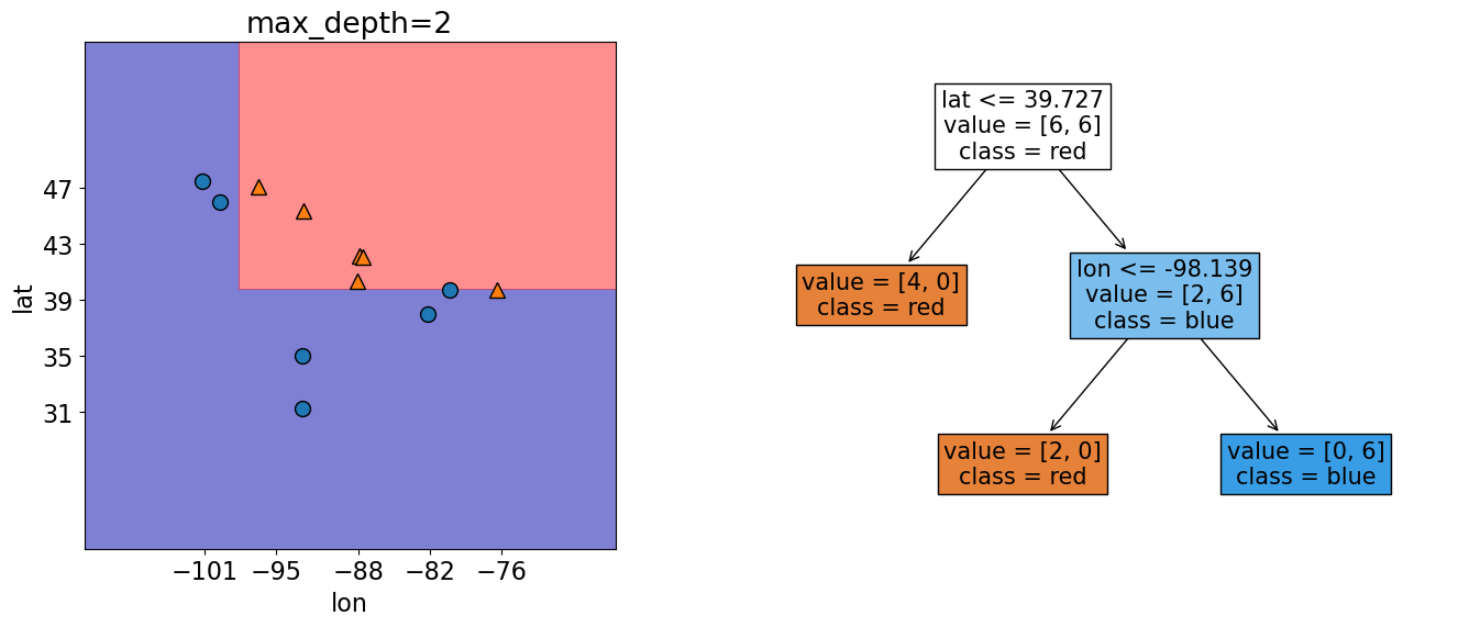
Let’s try growing a more complex tree model and now set max_depth = 2

model_2 = DecisionTreeClassifier(max_depth=2).fit(X, y)

plot_tree(
    model_2,
    feature_names=X.columns,
    class_names=y.unique()[::-1],
    impurity=False,
    ax=plt.subplots(figsize=(6, 6))[1]
);

This has 3 splits in the tree so we expect 3 decision boundaries (2 on lon and 1 on lat).

plot_tree_decision_boundary(
    model_2,
    X,
    y,
    eps=10,
    x_label="lon",
    y_label="lat",
)

Looking at the score of this model now get an accuracy of 100%!

model_2.score(X, y)

We see here that as max_depth increases, the accuracy of the training data does as well.

Doing this isn’t always the best idea and we’ll explain this a little bit later on.

This is just one of many other hyperparameters for decision trees that you can explore -> link here There are many other hyperparameters for decision trees that you can explore at the link here.

To summarize this section:

parameters are automatically learned by an algorithm during training
hyperparameters are specified before training

1.10. Decision Tree Regressor#

We saw that we can use decision trees for classification problems but we can also use this decision tree algorithm for regression problems.

Instead of using Gini impurity (which we briefly mentioned this above), we can use some other criteria for splitting.

(A common one is mean squared error (MSE) which we will discuss shortly)

scikit-learn supports regression using decision trees with DecisionTreeRegressor() and the .fit() and .predict() paradigm that is similar to classification.

Let’s do an example using the kc_house_data we saw in example 1.

df = pd.read_csv("data/kc_house_data.csv")
df = df.drop(columns=["id", "date"])
df

	price	bedrooms	bathrooms	sqft_living	sqft_lot	floors	waterfront	view	condition	grade	sqft_above	sqft_basement	yr_built	yr_renovated	zipcode	lat	long	sqft_living15	sqft_lot15
0	221900.0	3	1.00	1180	5650	1.0	0	0	3	7	1180	0	1955	0	98178	47.5112	-122.257	1340	5650
1	538000.0	3	2.25	2570	7242	2.0	0	0	3	7	2170	400	1951	1991	98125	47.7210	-122.319	1690	7639
2	180000.0	2	1.00	770	10000	1.0	0	0	3	6	770	0	1933	0	98028	47.7379	-122.233	2720	8062
3	604000.0	4	3.00	1960	5000	1.0	0	0	5	7	1050	910	1965	0	98136	47.5208	-122.393	1360	5000
4	510000.0	3	2.00	1680	8080	1.0	0	0	3	8	1680	0	1987	0	98074	47.6168	-122.045	1800	7503
...	...	...	...	...	...	...	...	...	...	...	...	...	...	...	...	...	...	...	...
21608	360000.0	3	2.50	1530	1131	3.0	0	0	3	8	1530	0	2009	0	98103	47.6993	-122.346	1530	1509
21609	400000.0	4	2.50	2310	5813	2.0	0	0	3	8	2310	0	2014	0	98146	47.5107	-122.362	1830	7200
21610	402101.0	2	0.75	1020	1350	2.0	0	0	3	7	1020	0	2009	0	98144	47.5944	-122.299	1020	2007
21611	400000.0	3	2.50	1600	2388	2.0	0	0	3	8	1600	0	2004	0	98027	47.5345	-122.069	1410	1287
21612	325000.0	2	0.75	1020	1076	2.0	0	0	3	7	1020	0	2008	0	98144	47.5941	-122.299	1020	1357

21613 rows × 19 columns

X = df.drop(columns=["price"])
X.head()

	bedrooms	bathrooms	sqft_living	sqft_lot	floors	condition	grade	sqft_above	sqft_basement	yr_built	yr_renovated	zipcode	lat	long	sqft_living15	sqft_lot15
0	3	1.00	1180	5650	1.0	3	7	1180	0	1955	0	98178	47.5112	-122.257	1340	5650
1	3	2.25	2570	7242	2.0	3	7	2170	400	1951	1991	98125	47.7210	-122.319	1690	7639
2	2	1.00	770	10000	1.0	3	6	770	0	1933	0	98028	47.7379	-122.233	2720	8062
3	4	3.00	1960	5000	1.0	5	7	1050	910	1965	0	98136	47.5208	-122.393	1360	5000
4	3	2.00	1680	8080	1.0	3	8	1680	0	1987	0	98074	47.6168	-122.045	1800	7503

y = df["price"]
y.head()

  221900.0
  538000.0
  180000.0
  604000.0
  510000.0
Name: price, dtype: float64

We can see that instead of predicting a categorical column like we did with vote before, our target column is now numeric.

Instead of importing DecisionTreeClassifier, we import DecisionTreeRegressor.

We follow the same steps as before and can even set hyperparameters as we did in classification.

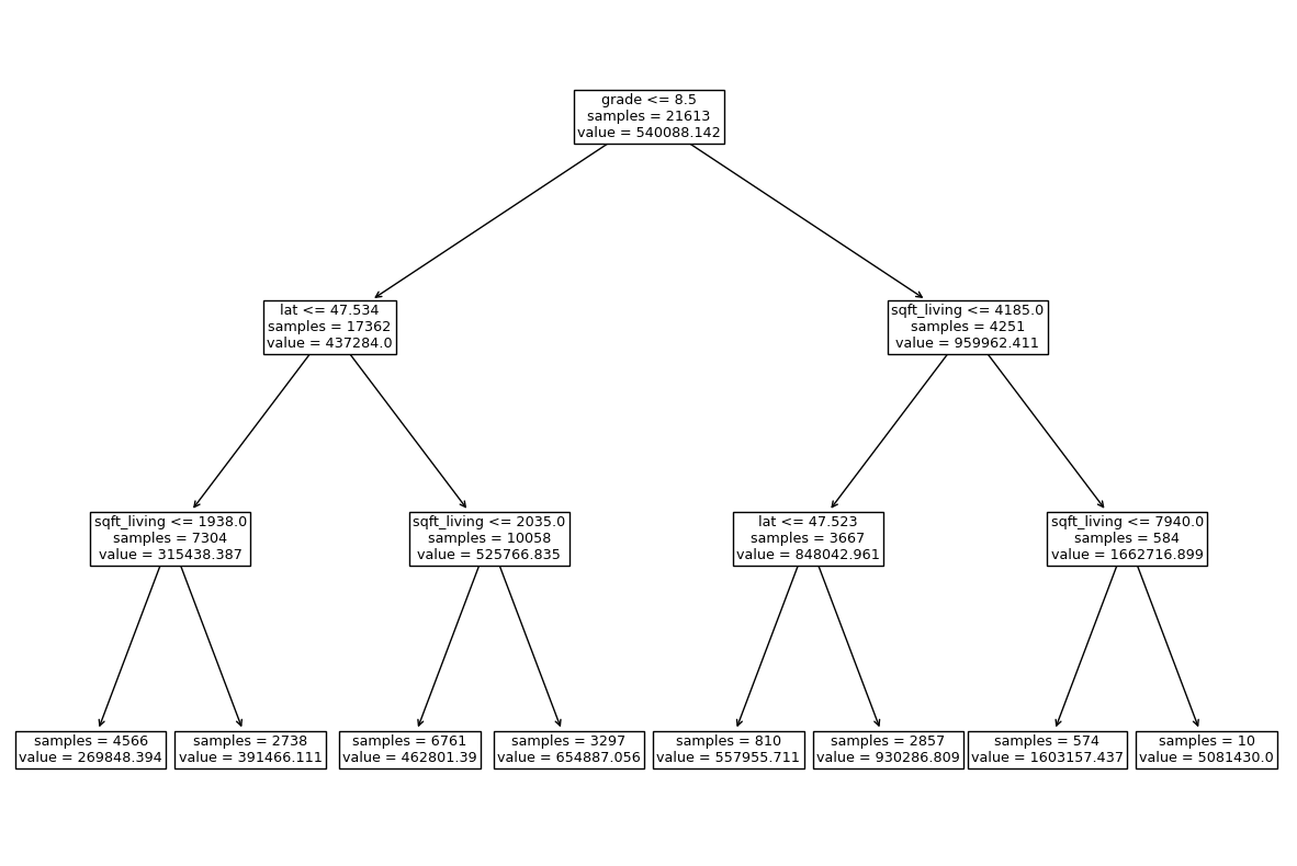
Here, when we build our model, we are specifying a max_depth of 3.

This means our decision tree is going to be constrained to a depth of 3.

from sklearn.tree import DecisionTreeRegressor

depth = 3
reg_model = DecisionTreeRegressor(max_depth=depth, random_state=1)
reg_model.fit(X, y)

DecisionTreeRegressor(max_depth=3, random_state=1)

In a Jupyter environment, please rerun this cell to show the HTML representation or trust the notebook.
On GitHub, the HTML representation is unable to render, please try loading this page with nbviewer.org.

Let’s look at the tree it produces our leaves used to contain a categorical value for prediction, but this time we see our leaves are predicting numerical values.

plot_tree(
    reg_model,
    feature_names=X.columns,
    impurity=False,
    ax=plt.subplots(figsize=(15, 10))[1]
);

Let’s see what our model predicts for a single example.

X.loc[[0]]

	bedrooms	bathrooms	sqft_living	sqft_lot	floors	waterfront	view	condition	grade	sqft_above	sqft_basement	yr_built	yr_renovated	zipcode	lat	long	sqft_living15	sqft_lot15
0	3	1.0	1180	5650	1.0	0	0	3	7	1180	0	1955	0	98178	47.5112	-122.257	1340	5650

reg_model.predict(X.loc[[0]])

array([269848.39378011])

Our model predicts a housing price of $269848.39

Should we see what the true value is?

y.loc[[0]]

0    221900.0
Name: price, dtype: float64

The true value is $221900.0, but how well did it score?

With regression problems we can’t use accuracy for a scoring method so instead when we use .score() it returns somethings called an 𝑅2 (r squared) score.

reg_model.score(X,y)

0.6069320183816143

The maximum 𝑅2 is 1 for perfect predictions, 0 means that the same value would be predicted regardless of the input value, and a negative value would mean that the model is performing worse than outputting a constant value (e.g. the higher the actual value, the lower the prediction is).

1.11. Let’s Practice - Coding#

Using the data candybars.csv from the datafolder (or going to exercise 7 here) for the following:

Define two objects named X and y which contain the features and target column respectively.
Using sklearn, create 3 different decision tree classifiers using 3 different min_samples_split values based on this data.
What is the accuracy of each classifier on the training data?
a) Which min_samples_split value would you choose to predict this data?
b) Would you choose the same min_samples_split value to predict new data?
Do you think most of the computational effort for a decision tree takes place in the .fit() stage or .predict() stage?

candy_df = pd.read_csv('data/candybars.csv', index_col=0)
candy_df

	chocolate	peanuts	caramel	nougat	cookie_wafer_rice	coconut	white_chocolate	multi	availability
candy bar
CoffeeCrisp	1	0	0	0	1	0	0	0	Canada
Butterfinger	1	1	1	0	0	0	0	0	America
Skor	1	0	1	0	0	0	0	0	Both
Smarties	1	0	0	0	0	0	0	1	Canada
Twix	1	0	1	0	1	0	0	1	Both
ReesesPeanutButterCups	1	1	0	0	0	0	0	1	Both
3Musketeers	1	0	0	1	0	0	0	0	America
Kinder Surprise	1	0	0	0	0	0	1	0	Canada
M&Ms	1	1	0	0	0	0	0	1	Both
Glosettes	1	0	0	0	0	0	0	1	Canada
KitKat	1	0	0	0	1	0	0	1	Both
Babe Ruth	1	1	1	1	0	0	0	0	America
Caramilk	1	0	1	0	0	0	0	0	Canada
Aero	1	0	0	0	0	0	0	0	Canada
Mars	1	0	1	1	0	0	0	0	Both
Payday	0	1	1	0	0	0	0	0	America
Snickers	1	1	1	1	0	0	0	0	Both
Crunchie	1	0	0	0	0	0	0	0	Canada
Wonderbar	1	1	1	0	0	0	0	0	Canada
100Grand	1	0	1	0	1	0	0	0	America
Take5	1	1	1	0	1	0	0	0	America
Whatchamacallits	1	1	0	0	1	0	0	0	America
AlmondJoy	1	0	0	0	0	1	0	0	America
OhHenry	1	1	1	0	0	0	0	0	Both
CookiesandCream	0	0	0	0	1	0	1	0	Both

Solutions

1.

X = candy_df.drop(columns='availability')
y = candy_df['availability']

y.head()

candy bar
CoffeeCrisp      Canada
Butterfinger    America
Skor               Both
Smarties         Canada
Twix               Both
Name: availability, dtype: object

2 and 3.

# 2/3.
dt2 = DecisionTreeClassifier(min_samples_split=5)
dt2.fit(X, y)
dt2.score(X, y)

0.72

X.columns

Index(['chocolate', 'peanuts', 'caramel', 'nougat', 'cookie_wafer_rice',
       'coconut', 'white_chocolate', 'multi'],
      dtype='object')

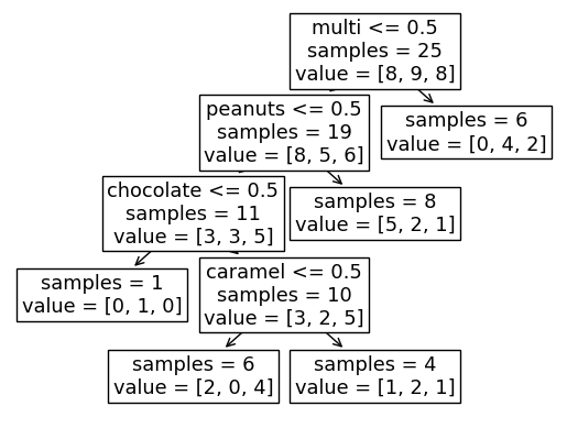
plot_tree(
    dt2,
    feature_names=X.columns,
    impurity=False,
    ax=plt.subplots(figsize=(15, 10))[1]
);

2 and 3.

# 2/3.
dt5 = DecisionTreeClassifier(min_samples_split=4)
dt5.fit(X, y)
dt5.score(X, y)

0.84

2 and 3.

# 2/3.
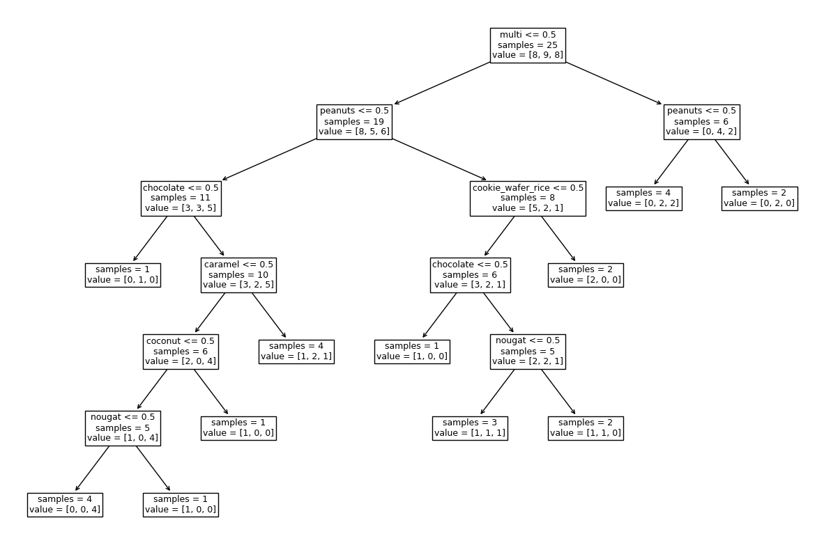
dt10 = DecisionTreeClassifier(min_samples_split=20)
dt10.fit(X, y)
dt10.score(X, y)

0.48

plot_tree(
    dt10,
    feature_names=X.columns,
    impurity=False,
#     ax=plt.subplots(figsize=(15, 10))[1]
);

4.

In this example, the best performance on the training data is given when min_samples_split=2. We don’t know if this generalizes best to predicting unseen data, and to find out we would need to evaluate the different hyperparameter values on a validation data set, ideally using cross-validation, which we will talk about next lecture.

5.

The fit stage is more computationally expensive since this is where the optimal feature splits are being computed. The predict stage is using these already created rules to classify new points.

1.12. What We’ve Learned Today #

What is machine learning (supervised/unsupervised, classification/regression)
Machine learning terminology
What is the decision tree algorithm and how does it work
The scikit-learn library
Parameters and hyperparameters

BAIT 509
Business Applications of Machine Learning

Intro to ML & Decision Trees

Contents

1. Intro to ML & Decision Trees#

1.1. Welcome#

1.1.1. Course Learning Objectives#

1.1.2. Python, Jupyter, Visualizations#

1.1.3. Lecture Learning Objectives#

1.2. What is Machine Learning (ML)?#

1.3. Types of Machine Learning#

1.3.1. Supervised Learning:#

1.3.2. UnSupervised Learning: (not going into detail here)#

1.4. Types of Supervised Learning: Classification vs Regression#

1.4.1. Classification#

1.4.2. Regression#

1.5. Let’s Practice#

1.6. Tabular Data and Terminology#

1.6.1. Example:#

1.7. Decision Tree Algorithm#

1.7.1. A conceptual introduction to Decision Trees#

1.7.2. Implimentation with Scikit-learn#

1.7.2.1. 1. Read the data#

1.7.2.2. 2. Create \(X\) and \(y\)#

1.7.2.3. 3. Create a classifier object#

1.7.2.4. 4. Fit the classifier#

1.7.2.5. 5. Predict the target using unseen data#

1.7.2.6. 6. Score the model#

1.8. Let’s Practice#

1.9. Parameters and Hyperparameters#

1.9.1. Parameters#

1.9.2. Hyperparameters#

1.10. Decision Tree Regressor#

1.11. Let’s Practice - Coding#

1.12. What We’ve Learned Today #

BAIT 509Business Applications of Machine Learning

Intro to ML & Decision Trees

Contents

1. Intro to ML & Decision Trees#

1.1. Welcome#

1.1.1. Course Learning Objectives#

1.1.2. Python, Jupyter, Visualizations#

1.1.3. Lecture Learning Objectives#

1.2. What is Machine Learning (ML)?#

1.3. Types of Machine Learning#

1.3.1. Supervised Learning:#

1.3.2. UnSupervised Learning: (not going into detail here)#

1.4. Types of Supervised Learning: Classification vs Regression#

1.4.1. Classification#

1.4.2. Regression#

1.5. Let’s Practice#

1.6. Tabular Data and Terminology#

1.6.1. Example:#

1.7. Decision Tree Algorithm#

1.7.1. A conceptual introduction to Decision Trees#

1.7.2. Implimentation with Scikit-learn#

1.7.2.1. 1. Read the data#

1.7.2.2. 2. Create \(X\) and \(y\)#

1.7.2.3. 3. Create a classifier object#

1.7.2.4. 4. Fit the classifier#

1.7.2.5. 5. Predict the target using unseen data#

1.7.2.6. 6. Score the model#

1.8. Let’s Practice#

1.9. Parameters and Hyperparameters#

1.9.1. Parameters#

1.9.2. Hyperparameters#

1.10. Decision Tree Regressor#

1.11. Let’s Practice - Coding#

1.12. What We’ve Learned Today#

BAIT 509
Business Applications of Machine Learning

1.12. What We’ve Learned Today #