Business Objectives/Statistical Questions and Feature Selection
Contents
8. Business Objectives/Statistical Questions and Feature Selection#
8.1. Lecture Learning Objectives#
In the context of supervised learning, form statistical questions from business questions/objectives.
Understand the different forms your client may expect you to communicate results.
Explain the general concept of feature selection.
Discuss and compare different feature selection methods at a high level.
Use sklearn’s implementation of recursive feature elimination (RFE).
Implement the forward search algorithm.
8.2. Five Minute Recap/ Lightning Questions#
What is the hyperparameter we learned for Ridge and how does it affect the Fundamental Trade-off?
What is the hyperparameter we learned for Logistic Regression and how does it affect the Fundamental Trade-off?
What is the name of the function used to bound our values between 0 and 1
What is the name of the function that gives “hard” predictions?
What is the name of the function that gives “soft” predictions?
8.2.1. Some lingering questions#
How can we start forming good business questions that can be addressed with Machine Learning?
Is the best model always the one with all the features? If not, how to select features for our models?
8.3. Forming statistical questions to answer business objectives#
So far you’ve seen how to solve predictive problems using machine learning but today, we are going to look at the process involved in asking the questions and problems faced by organizations.
Generally, there are four parts of a machine learning analysis. In order from high to low level:
The business question/objective
The statistical question/objective
The data and model
The data product
Doing a machine learning analysis is about distilling from the highest level to the lowest level. As such, there are three distillations to keep in mind: 1-2, 2-3, and 3-4:
1-2 is about asking the right questions
2-3 is about building a useful model
3-4 is about communicating the results
Note that an analysis isn’t a linear progression through these “steps”; rather, the process is iterative. This is because none of the components are independent. Making progress on any of the three distillations gives you more information as to what the problem is.
We’ll look at each of these distillations in turn.
8.4. (1 - 2) Asking useful statistical questions#
Usually, a company is not served up a machine learning problem, complete with data and a description of the response and predictors.
Companies don’t exactly know what question is the right question but they do know what they want to be accomplished.
Instead, they’re faced with some high-level objective/question that we’ll call the business question/objective.
This question needs refining to a statistical question/objective – one that is directly addressable by machine learning.
8.4.1. Business objectives: examples#
This altexsoft blog post is a great introduction to business use cases of data science/ML
Examples of business objectives (for which machine learning is a relevant approach)
Reduce the amount of spam email received
Early prediction of product failure
Find undervalued mines
Make a transit system more efficient
Hire efficient staff
Predict Customer Lifetime Value
Understand Sales performance
Fraud detection
8.4.2. Refining business objectives to statistical objectives#
Statistical objectives need to be specific
Remember that supervised learning is about predicting a response \(Y\) from predictors \(X_1,…,X_p\)
So we need to refine our business objectives to a statistical question(s) we can answer
This typically involves:
Identifying the response variable (\(Y\)) that is most aligned with the business objective.
Identifying the data (observations + features) that will be used for model development/testing.
Note: part of this is the task of feature selection via machine learning methods – but this is also a human decision based on what we think is more informative, as well as a resource questions (what data is actually available?)
8.4.3. Statistical objectives: examples#
Statistical objectives corresponding to the above business objective examples might be:
Business Objective |
Statistical Question |
|---|---|
Reduce the amount of spam email received |
|
Early prediction of product failure (Kickstarter?) |
|
Find undervalued mines |
|
Make a transit system more efficient |
|
Hire efficient staff |
|
8.4.4. Statistical questions are not the full picture!#
Almost always, the business objective is more complex than the statistical question.
By refining a business objective to a statistical one, we may lose part of the essence of the business objective.
It’s important to have a sense of the ways in which your statistical objective falls short, and the ways in which it’s on the mark, so that you keep an idea of the big picture.
For example, predicting whether a new staff hire will be efficient or not is a useful statistical question, but doesn’t consider why a company might be attracting certain applicants, how long staff will remain, how staff work together, etc.
8.5. (2 - 3) Building a useful model#
This is the main focus of BAIT509.
This involves using ML algorithms (kNN, loess, decision trees, etc) to build a predictive model from data
You always should include a baseline model to assess how well the models you build are giving you some leg up.
Remember that a simple model like logistic regression often does as well as more complex approaches, and has the advantage that it is easier to explain. At the very least, simpler models can help guide you on what more complex approaches to take next, and provide another baseline so that you can assess if a more complex and harder to explain model is worthwhile.
8.6. (3 - 4) Communicating results#
So you’ve distilled your business objectives to a statistical question.
You’ve developed a model to answer the statistical question.
Now your model needs to be delivered and used by others (or your future self)!
The final delivery is often called “the data product” because it may consist of a variety of things:
a report
a presentation
an app
a dashboard
a software package/pipeline
Sometimes the client requests a specific data product -> But note that their suggestion might not always be the best option.
Perhaps they request a report and presentation communicating your findings, when a more appropriate product also includes an interactive app that allows them to explore your findings for themselves.
Either way, the key here is communication. Two import challenges (relevant to your final project):
Using appropriate language: there is a lot of jargon in ML, the key is to talk more about the output and the general idea of your model(s), but not machine learning or statistical jargon.
Communication with visual design: this is about choosing what visuals are the most effective for communicating. -> Plug: https://viz-learn.mds.ubc.ca/en/
Usually, the first step is to set up a framework for your data product. For a report, this means outlining what you intend to write about, and where.
Iterating with your client is useful to make sure that you are on track to produce something that the client currently sees as being potentially useful.
Don’t waste your time by working for months on your own and then realizing your misunderstood the ask when you are showing your final product.
It is easy to get lost in finding the coolest model or using the latest ML technique, and forget about the overarching question and the purpose of your analysis.
Take a step back and look at the big picture.
Adapt the mind-set of a researcher rather than an ML engineer.
How can I best help the client?
8.7. Let’s Practice#
What question is usually more complex: The business or statistical one?
What model needs to be made for all problems to create a baseline?
In supervised learning, once we have our business objective, part of our statistical question is identifying what?
True or False:
When writing your reports, it’s important to consider who is reading it.
Sometimes you may need to dig a little to figure out exactly what the client wants.
In supervised learning, we should take into consideration the uncertainty of our models.
Solutions!
Business question/objective
Baseline - Dummy
Our target variable
True
True
True
8.8. Feature Selection#
8.8.1. Motivation#
Remember the curse of dimensionality?
We spoke about this briefly when we discussed \(k\)-nn and how when we add many different dimensions (features) it makes the data more sparse since the ratio of observations to features/dimensions goes down. This can make it harder for the model to learn which features are relevant to predict the outcome, since there is now a lower density of training samples to query. With many irrelevant features, the model can disintegrate towards predictions no better than random guessing.
Another drawback with a model that has many features is that it can be harder to interpret and explain what is important in the model’s decision making.
Reasons like this are why we need to be careful about which features we include in our model.
8.8.2. How do we limit the number of features in our model#
Use domain knowledge and manually select features (often in combination with one of the approaches below).
We could systematically rearrange and drop features to create one dataset for each possible combination/permutation of features. Then we would have a score for each possible feature combination and we could compare which features are the most important for model accuracy. Although this makes sense conceptually, it is practically infeasible since we would have feature factorial (often written as \(p!\)) as the number of datasets and on each dataset we would also need to perform a hyperparameter search. This would take too long for most real world datasets.
We could use machine learning to identify which features are important. For example, we talked about how lasso regression tries to bring some coefficients to 0, which means we can remove them from the model. This could be used as a preprocessing step before fitting another model on the selected features.
We could compute some type of score for how important a feature is for the model prediction, and then drop features under a threshold.
We will mostly talk about point 4 in this lecture.
8.8.3. What is an important feature?#
There are several definitions of how to measure how important a feature is. We have already seen that in scaled data, the magnitude of the coefficients in a linear regression can indicate how much the predicted value change when the value of that feature changes; this is one type of indication of the importance of that feature. But what can we do for models that don’t have coefficients, such as decision trees?
Decision trees actually have a built in feature importance estimate. Recall that the splits in a decision tree are chosen to maximize the homogeneity in each of the groups remaining after the split. Another way of saying this, is that “impurity” of the sample is decreasing with each split . The built-in decision tree feature importance is based on the total decrease in impurity from all nodes/splits of a particular feature, weighted by the number of samples that reach these nodes/splits. Features used at the top of the tree contribute to the final prediction decision of a larger fraction of the input samples and therefore often have a higher contribution to the decrease in impurity (a high feature importance).
You can think of “impurity” here in a colloquial sense of the word. Technically it is defined as proportion of mislabeled observations in a node if we were to label the observations at random based on the occurrence of each class among the observations in that node. Impurity is 0 when all observations in the node come from the same class.
8.8.4. Feature importance#
We can find out which features are most important in a decision tree model using an attribute called feature_importances_.
import pandas as pd
from sklearn.model_selection import train_test_split


cities_df = pd.read_csv("data/canada_usa_cities.csv")
train_df, test_df = train_test_split(cities_df, test_size=0.2, random_state=123)
X_train, y_train = train_df.drop(columns=["country"], axis=1), train_df["country"]
X_test, y_test = test_df.drop(columns=["country"], axis=1), test_df["country"]

train_df.head()
| longitude | latitude | country | |
|---|---|---|---|
| 160 | -76.4813 | 44.2307 | Canada |
| 127 | -81.2496 | 42.9837 | Canada |
| 169 | -66.0580 | 45.2788 | Canada |
| 188 | -73.2533 | 45.3057 | Canada |
| 187 | -67.9245 | 47.1652 | Canada |
from sklearn.tree import DecisionTreeClassifier


dt_model = DecisionTreeClassifier(max_depth=5)
dt_model.fit(X_train, y_train)
dt_model.feature_importances_
array([0.27718465, 0.72281535])
We can use the .feature_importances_ attribute to see the decrease in impurity.
A higher value = a more important features.
X_train.columns
Index(['longitude', 'latitude'], dtype='object')
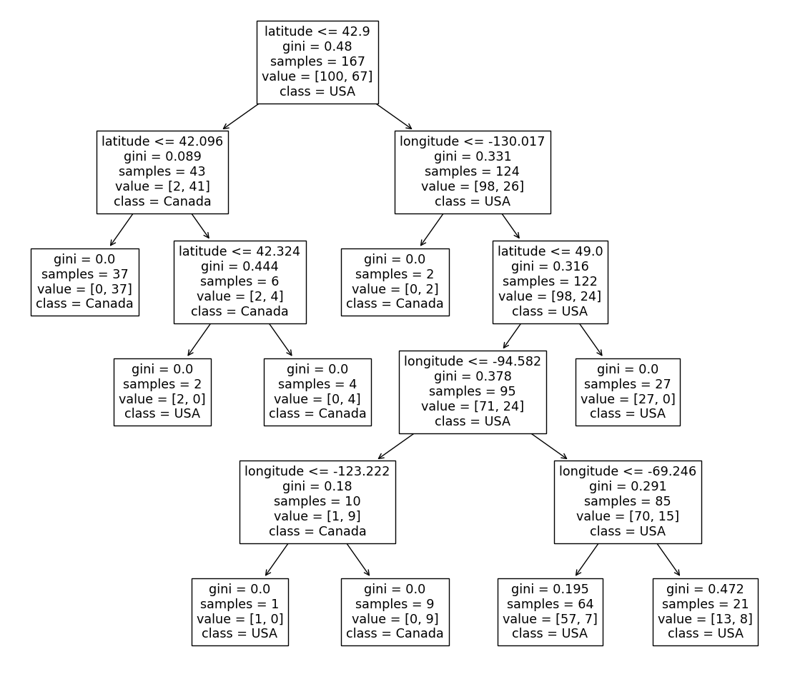
Here we can see that most of the importance is on the column latitude,
which makes sense since USA and Canada are separated mainly in latitude.
If we graph this, the root of the decision tree will usually reflect the top feature. Just like we can see here (here we also include the impurity of each node, called “gini”):
from sklearn.tree import plot_tree
import matplotlib.pyplot as plt


plot_tree(
    dt_model,
    feature_names=X_train.columns,
    class_names=y_train.unique()[::-1],
    impurity=True,
    ax=plt.subplots(figsize=(14, 12))[1]  # We need to create a figure to control the overall plot size
);
8.9. Are impurity based features importances reliable?#
Betteridge’s law of headlines: “Any headline that ends in a question mark can be answered by the word no.” As is the case here. The default feature importance calculated by decisions trees is not always reliable and tend to give too high weight to features with many unique values. Let’s see an example using a dataset from the passengers of the Titanic.
# Example adapted from https://scikit-learn.org/stable/auto_examples/inspection/plot_permutation_importance.html

from sklearn.datasets import fetch_openml
import numpy as np

X, y = fetch_openml("titanic", version=1, as_frame=True, return_X_y=True)
rng = np.random.RandomState(seed=42)
X["random_cat"] = rng.randint(3, size=X.shape[0])
X["random_num"] = rng.randn(X.shape[0])

categorical_columns = ["pclass", "sex", "embarked", "random_cat"]
numerical_columns = ["age", "sibsp", "parch", "fare", "random_num"]

X = X[categorical_columns + numerical_columns]

X_train, X_test, y_train, y_test = train_test_split(X, y, stratify=y, random_state=42)
X_train
/Users/quannguyen/opt/miniconda3/envs/571/lib/python3.10/site-packages/sklearn/datasets/_openml.py:1022: FutureWarning: The default value of `parser` will change from `'liac-arff'` to `'auto'` in 1.4. You can set `parser='auto'` to silence this warning. Therefore, an `ImportError` will be raised from 1.4 if the dataset is dense and pandas is not installed. Note that the pandas parser may return different data types. See the Notes Section in fetch_openml's API doc for details.
  warn(
| pclass | sex | embarked | random_cat | age | sibsp | parch | fare | random_num | |
|---|---|---|---|---|---|---|---|---|---|
| 1216 | 3.0 | female | Q | 1 | NaN | 0.0 | 0.0 | 7.7333 | -0.436386 |
| 819 | 3.0 | female | Q | 2 | NaN | 0.0 | 0.0 | 7.7500 | 2.006093 |
| 1286 | 3.0 | female | C | 2 | 38.0 | 0.0 | 0.0 | 7.2292 | 0.521122 |
| 1280 | 3.0 | male | S | 1 | 22.0 | 0.0 | 0.0 | 7.8958 | -2.135674 |
| 761 | 3.0 | male | S | 0 | 16.0 | 0.0 | 0.0 | 9.5000 | 1.607346 |
| ... | ... | ... | ... | ... | ... | ... | ... | ... | ... |
| 872 | 3.0 | female | S | 0 | NaN | 0.0 | 0.0 | 8.0500 | 0.766080 |
| 777 | 3.0 | male | S | 0 | 19.0 | 0.0 | 0.0 | 8.0500 | 2.601683 |
| 423 | 2.0 | male | S | 0 | 34.0 | 0.0 | 0.0 | 13.0000 | 0.346488 |
| 668 | 3.0 | male | S | 0 | 22.0 | 0.0 | 0.0 | 8.0500 | 0.949554 |
| 2 | 1.0 | female | S | 2 | 2.0 | 1.0 | 2.0 | 151.5500 | 0.935678 |
981 rows × 9 columns
We have added two random columns to the data, ideally they should have near 0 feature importance, since they are just assigned a random value by us and thus have no predictive value.
y is whether the passenger survived the titanic or not.
y
0       1
1       1
2       0
3       0
4       0
       ..
1304    0
1305    0
1306    0
1307    0
1308    0
Name: survived, Length: 1309, dtype: category
Categories (2, object): ['0', '1']
Create a decision tree pipeline with some preprocessing.
from sklearn.preprocessing import OneHotEncoder
from sklearn.compose import ColumnTransformer
from sklearn.pipeline import Pipeline
from sklearn.tree import DecisionTreeClassifier
from sklearn.impute import SimpleImputer


categorical_encoder = OneHotEncoder(handle_unknown="ignore")
numerical_pipe = Pipeline([("imputer", SimpleImputer(strategy="mean"))])

preprocessing = ColumnTransformer(
    [
        ("cat", categorical_encoder, categorical_columns),
        ("num", numerical_pipe, numerical_columns),
    ]
)

pipe = Pipeline(
    [
        ("preprocess", preprocessing),
        ("classifier", DecisionTreeClassifier(random_state=42)),
    ]
)
pipe.fit(X_train, y_train)
pipe.score(X_train, y_train)
1.0
pipe.named_steps["classifier"].get_depth()
22
pipe.score(X_test, y_test)
0.7530487804878049
We can use the .feature_importances_ attribute to see the mean decrease in impurity.
A higher value = a more important features.
pipe.named_steps["classifier"].feature_importances_
array([0.01654092, 0.        , 0.06896032, 0.        , 0.26473697,
       0.00758303, 0.00801158, 0.0102391 , 0.0161727 , 0.00590995,
       0.01372136, 0.15099661, 0.0381931 , 0.0167087 , 0.16208436,
       0.2201413 ])
Let’s plot them instead so it is easier to see.
import matplotlib.pyplot as plt


ohe = pipe.named_steps["preprocess"].named_transformers_["cat"]
feature_names = ohe.get_feature_names_out(categorical_columns)
feature_names = np.r_[feature_names, numerical_columns]

tree_feature_importances = pipe.named_steps["classifier"].feature_importances_
sorted_idx = tree_feature_importances.argsort()[::-1]

y_ticks = np.arange(0, len(feature_names))
fig, ax = plt.subplots(figsize=(10, 6))
ax.barh(y_ticks, tree_feature_importances[sorted_idx])
ax.set_yticks(y_ticks)
ax.set_yticklabels(feature_names[sorted_idx])
ax.set_title("Feature Importances (MDI)")
fig.tight_layout()
plt.show()
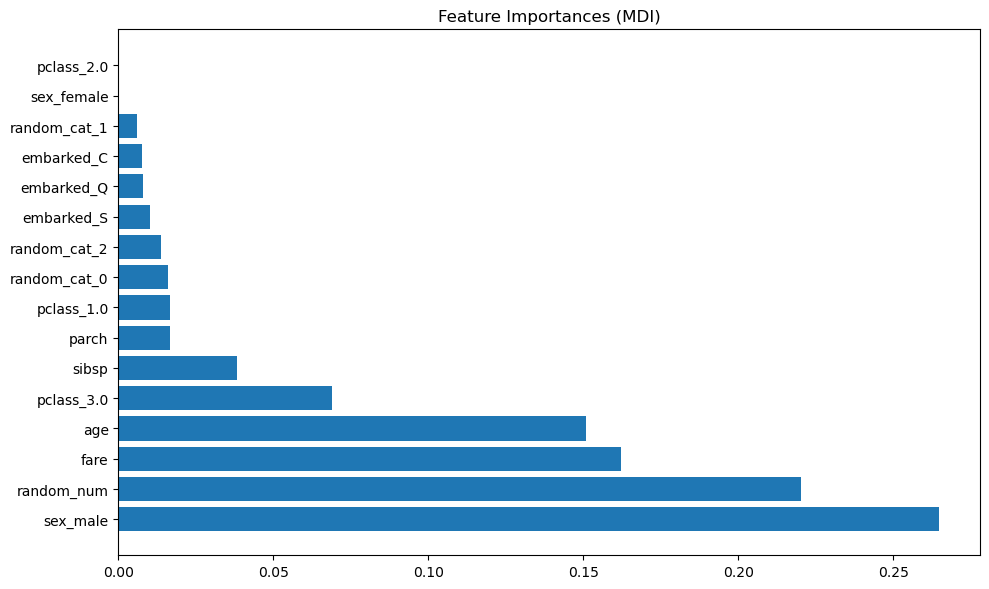
The impurity-based feature importance ranks the numerical features to be the most important features. As a result, the non-predictive random_num variable is ranked the second most important!
This problem stems from two limitations of impurity-based feature importances:
impurity-based importances are biased towards high cardinality features (features with many unique values)
You can think of this as a feature with many unique values will be part of many splits in the decision tree (although with few samples). Limiting the depth of the decision tree can reduce this effect, but might lead to underfitting instead.
impurity-based importances are computed on training set statistics and therefore do not reflect the ability of feature to be useful to make predictions that generalize to the test set.
A reminder about binary OneHotEncoded features is that only one of them is useful.
You can see here that all the information contained in sex_male and sex_female is the same,
and although this is very predictive of the survival outcome,
the model only needed one of them (the other has 0 feature importance).
Also note that just because the column is called
sex_male, it doesn’t mean that males had a higher chance of survival. Remember that this feature is encoded as 0 and 1 so it contains information about males and females. In fact, a much higher proportion of the female passengers survived the Titanic:
X_train.join(y).groupby('sex')['survived'].value_counts(normalize=True, sort=False)
/var/folders/q8/b0hct6591d77ky6m9kfk2jhw0000gp/T/ipykernel_11687/3116214982.py:1: FutureWarning: The default of observed=False is deprecated and will be changed to True in a future version of pandas. Pass observed=False to retain current behavior or observed=True to adopt the future default and silence this warning.
  X_train.join(y).groupby('sex')['survived'].value_counts(normalize=True, sort=False)
sex     survived
female  0           0.278261
        1           0.721739
male    0           0.801887
        1           0.198113
Name: proportion, dtype: float64
8.9.1. Permutation importances as an alternative to impurity-based feature importances#
From https://christophm.github.io/interpretable-ml-book/feature-importance.html
The concept is really straightforward: We measure the importance of a feature by calculating the increase in the model’s prediction error after permuting the feature. A feature is “important” if shuffling its values increases the model error, because in this case the model relied on the feature for the prediction. A feature is “unimportant” if shuffling its values leaves the model error unchanged, because in this case the model ignored the feature for the prediction. The permutation feature importance measurement was introduced by Breiman (2001)43 for random forests
Permutation importances can also be computed on the test/validation set to show what was most useful for the model in making predictions on unseen data.
from sklearn.inspection import permutation_importance


result = permutation_importance(
    pipe, X_test, y_test, n_repeats=10, random_state=42,
)
result
{'importances_mean': array([ 0.09603659,  0.14268293,  0.01981707, -0.00579268,  0.03993902,
         0.01219512,  0.00243902,  0.02987805,  0.00213415]),
 'importances_std': array([0.01280851, 0.02115775, 0.01092893, 0.00877816, 0.01949551,
        0.00304878, 0.00404466, 0.01529261, 0.00862864]),
 'importances': array([[ 0.11280488,  0.1097561 ,  0.10060976,  0.10060976,  0.09146341,
          0.1097561 ,  0.09756098,  0.07926829,  0.08536585,  0.07317073],
        [ 0.11890244,  0.14939024,  0.17682927,  0.17378049,  0.13719512,
          0.10670732,  0.12804878,  0.1554878 ,  0.13719512,  0.14329268],
        [ 0.00609756,  0.02743902,  0.01829268,  0.03963415,  0.        ,
          0.01829268,  0.02439024,  0.02439024,  0.02743902,  0.01219512],
        [-0.01219512,  0.00304878,  0.00304878, -0.00609756, -0.00914634,
         -0.02134146,  0.00304878, -0.01829268,  0.00304878, -0.00304878],
        [ 0.03353659,  0.03963415,  0.04268293,  0.04268293,  0.05182927,
          0.08536585,  0.04573171,  0.01829268,  0.0304878 ,  0.00914634],
        [ 0.00914634,  0.01219512,  0.0152439 ,  0.0152439 ,  0.01829268,
          0.00914634,  0.00914634,  0.01219512,  0.00914634,  0.01219512],
        [ 0.00304878,  0.        ,  0.00914634,  0.00609756,  0.00914634,
          0.        ,  0.        ,  0.        , -0.00304878,  0.        ],
        [ 0.03963415,  0.04878049,  0.04268293,  0.04268293,  0.0304878 ,
          0.03353659,  0.00304878,  0.0152439 ,  0.00609756,  0.03658537],
        [ 0.02134146, -0.00304878,  0.        , -0.00609756,  0.        ,
          0.00304878,  0.        , -0.00304878,  0.0152439 , -0.00609756]])}
Let’s visualize the results.
sorted_idx = result.importances_mean.argsort()
fig, ax = plt.subplots(figsize=(8, 6))
ax.boxplot(result.importances[sorted_idx].T, vert=False, labels=X_test.columns[sorted_idx])
ax.set_title("Permutation Importances (test set)")
ax.set_xlabel("Model error increase when the feature was permutated")
fig.tight_layout()
plt.show()
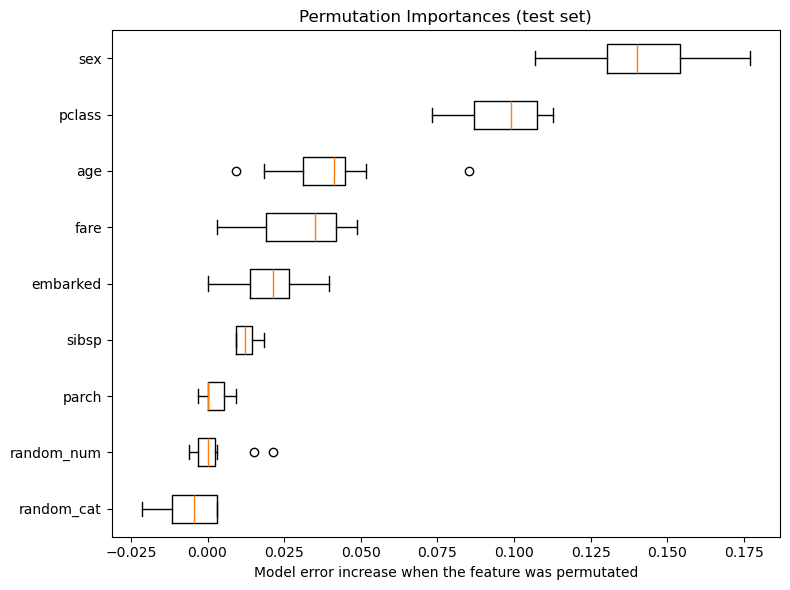
This shows that the low cardinality categorical feature, sex is the most important feature, and passenger class affect the model error more than both age and fare. Also note that both random features have very low importances (close to 0) as expected.
Note Remember that explaining the model \(\neq\) explaining the data. Especially if we have a badly performing model, it might not matter that much to us what the most important features are and they might be quite different for a model that performs well.
Once we have found a feature importance score that we think is useful for our application, we could simply set a threshold for what should be included. This threshold might be specific for our application and could for example be “Select feature that contribute more than 5% to the model error”. We could also have a pre-determined number of features we want to select or look for a drastic change in the plot. Above it looks like the top two features are quite more important than the rest.
However, although these plots can be informative for the importance of features in models where they are all included, it doesn’t really tell us how well a model with only the most important features will perform. Are we missing some interaction with the other features so that our model will fewer feature will score worse? Or are the other features mostly adding noise, so that our model will fewer features will score better? To find out, we would still need to score the model with a different amount of features, but now that we have an indication of how important the features are, we can use this info to tell us which ones to start removing.
8.9.2. Recursive feature elimination - RFE#
The basic idea with recursive feature elimination is that we remove features according to the following steps:
We decide \(k\) - the number of features to select.
Assign importances to features, e.g. by fitting a model and looking at coef_ or feature_importances_.
Remove the least important feature.
Repeat steps 2-3 until only \(k\) features are remaining.
Note This is not the same as just removing all the less important features in one shot. Here we actually evaluate each model to see if it is getting better or worse.
Unfortunately,
RFE does currently not work with permutation importances in sklearn (yet),
so we would have to use models with built-in feature importances,
such as those in .coef_ or .feature_importances_.
Here we will fit a logistic regression model
and show how we can use its coefficients in RFE to select features.
8.9.3. New housing data#
I know at this point you are probably annoyed and bored of housing data, but good, interesting open-source data is hard to come by. For this example, I really want to show you an example with LOTS of features.
Here is (yet another) housing dataset we acquired from this GitHub repo, originally created by Dean De Cock. (We are using the raw data so we do not need to store it and import it simply from the url.)
Attribution:
The Ames Housing dataset was compiled by Dean De Cock for use in data science education.
His publication can be found here.
ames_df = pd.read_csv('https://raw.githubusercontent.com/melindaleung/Ames-Iowa-Housing-Dataset/master/data/ames%20iowa%20housing.csv', index_col=0)
ames_df.loc[ames_df['SaleCondition'] != 'Normal', 'SaleCondition'] = 'Abnormal'
ames_df
| MSSubClass | MSZoning | LotFrontage | LotArea | Street | Alley | LotShape | LandContour | Utilities | LotConfig | ... | PoolArea | PoolQC | Fence | MiscFeature | MiscVal | MoSold | YrSold | SaleType | SaleCondition | SalePrice | |
|---|---|---|---|---|---|---|---|---|---|---|---|---|---|---|---|---|---|---|---|---|---|
| Id | |||||||||||||||||||||
| 1 | 60 | RL | 65.0 | 8450 | Pave | NaN | Reg | Lvl | AllPub | Inside | ... | 0 | NaN | NaN | NaN | 0 | 2 | 2008 | WD | Normal | 208500 |
| 2 | 20 | RL | 80.0 | 9600 | Pave | NaN | Reg | Lvl | AllPub | FR2 | ... | 0 | NaN | NaN | NaN | 0 | 5 | 2007 | WD | Normal | 181500 |
| 3 | 60 | RL | 68.0 | 11250 | Pave | NaN | IR1 | Lvl | AllPub | Inside | ... | 0 | NaN | NaN | NaN | 0 | 9 | 2008 | WD | Normal | 223500 |
| 4 | 70 | RL | 60.0 | 9550 | Pave | NaN | IR1 | Lvl | AllPub | Corner | ... | 0 | NaN | NaN | NaN | 0 | 2 | 2006 | WD | Abnormal | 140000 |
| 5 | 60 | RL | 84.0 | 14260 | Pave | NaN | IR1 | Lvl | AllPub | FR2 | ... | 0 | NaN | NaN | NaN | 0 | 12 | 2008 | WD | Normal | 250000 |
| ... | ... | ... | ... | ... | ... | ... | ... | ... | ... | ... | ... | ... | ... | ... | ... | ... | ... | ... | ... | ... | ... |
| 1456 | 60 | RL | 62.0 | 7917 | Pave | NaN | Reg | Lvl | AllPub | Inside | ... | 0 | NaN | NaN | NaN | 0 | 8 | 2007 | WD | Normal | 175000 |
| 1457 | 20 | RL | 85.0 | 13175 | Pave | NaN | Reg | Lvl | AllPub | Inside | ... | 0 | NaN | MnPrv | NaN | 0 | 2 | 2010 | WD | Normal | 210000 |
| 1458 | 70 | RL | 66.0 | 9042 | Pave | NaN | Reg | Lvl | AllPub | Inside | ... | 0 | NaN | GdPrv | Shed | 2500 | 5 | 2010 | WD | Normal | 266500 |
| 1459 | 20 | RL | 68.0 | 9717 | Pave | NaN | Reg | Lvl | AllPub | Inside | ... | 0 | NaN | NaN | NaN | 0 | 4 | 2010 | WD | Normal | 142125 |
| 1460 | 20 | RL | 75.0 | 9937 | Pave | NaN | Reg | Lvl | AllPub | Inside | ... | 0 | NaN | NaN | NaN | 0 | 6 | 2008 | WD | Normal | 147500 |
1460 rows × 80 columns
ames_df.info()
<class 'pandas.core.frame.DataFrame'>
Index: 1460 entries, 1 to 1460
Data columns (total 80 columns):
 #   Column         Non-Null Count  Dtype
---  ------         --------------  -----
 0   MSSubClass     1460 non-null   int64
 1   MSZoning       1460 non-null   object
 2   LotFrontage    1201 non-null   float64
 3   LotArea        1460 non-null   int64
 4   Street         1460 non-null   object
 5   Alley          91 non-null     object
 6   LotShape       1460 non-null   object
 7   LandContour    1460 non-null   object
 8   Utilities      1460 non-null   object
 9   LotConfig      1460 non-null   object
 10  LandSlope      1460 non-null   object
 11  Neighborhood   1460 non-null   object
 12  Condition1     1460 non-null   object
 13  Condition2     1460 non-null   object
 14  BldgType       1460 non-null   object
 15  HouseStyle     1460 non-null   object
 16  OverallQual    1460 non-null   int64
 17  OverallCond    1460 non-null   int64
 18  YearBuilt      1460 non-null   int64
 19  YearRemodAdd   1460 non-null   int64
 20  RoofStyle      1460 non-null   object
 21  RoofMatl       1460 non-null   object
 22  Exterior1st    1460 non-null   object
 23  Exterior2nd    1460 non-null   object
 24  MasVnrType     588 non-null    object
 25  MasVnrArea     1452 non-null   float64
 26  ExterQual      1460 non-null   object
 27  ExterCond      1460 non-null   object
 28  Foundation     1460 non-null   object
 29  BsmtQual       1423 non-null   object
 30  BsmtCond       1423 non-null   object
 31  BsmtExposure   1422 non-null   object
 32  BsmtFinType1   1423 non-null   object
 33  BsmtFinSF1     1460 non-null   int64
 34  BsmtFinType2   1422 non-null   object
 35  BsmtFinSF2     1460 non-null   int64
 36  BsmtUnfSF      1460 non-null   int64
 37  TotalBsmtSF    1460 non-null   int64
 38  Heating        1460 non-null   object
 39  HeatingQC      1460 non-null   object
 40  CentralAir     1460 non-null   object
 41  Electrical     1459 non-null   object
 42  1stFlrSF       1460 non-null   int64
 43  2ndFlrSF       1460 non-null   int64
 44  LowQualFinSF   1460 non-null   int64
 45  GrLivArea      1460 non-null   int64
 46  BsmtFullBath   1460 non-null   int64
 47  BsmtHalfBath   1460 non-null   int64
 48  FullBath       1460 non-null   int64
 49  HalfBath       1460 non-null   int64
 50  BedroomAbvGr   1460 non-null   int64
 51  KitchenAbvGr   1460 non-null   int64
 52  KitchenQual    1460 non-null   object
 53  TotRmsAbvGrd   1460 non-null   int64
 54  Functional     1460 non-null   object
 55  Fireplaces     1460 non-null   int64
 56  FireplaceQu    770 non-null    object
 57  GarageType     1379 non-null   object
 58  GarageYrBlt    1379 non-null   float64
 59  GarageFinish   1379 non-null   object
 60  GarageCars     1460 non-null   int64
 61  GarageArea     1460 non-null   int64
 62  GarageQual     1379 non-null   object
 63  GarageCond     1379 non-null   object
 64  PavedDrive     1460 non-null   object
 65  WoodDeckSF     1460 non-null   int64
 66  OpenPorchSF    1460 non-null   int64
 67  EnclosedPorch  1460 non-null   int64
 68  3SsnPorch      1460 non-null   int64
 69  ScreenPorch    1460 non-null   int64
 70  PoolArea       1460 non-null   int64
 71  PoolQC         7 non-null      object
 72  Fence          281 non-null    object
 73  MiscFeature    54 non-null     object
 74  MiscVal        1460 non-null   int64
 75  MoSold         1460 non-null   int64
 76  YrSold         1460 non-null   int64
 77  SaleType       1460 non-null   object
 78  SaleCondition  1460 non-null   object
 79  SalePrice      1460 non-null   int64
dtypes: float64(3), int64(34), object(43)
memory usage: 923.9+ KB
Here, we use .info() to identify our categorical and numeric features. I split my features and identify my target.
The target variable for this question is SaleCondition and we are doing classification.
train_df, test_df = train_test_split(ames_df, test_size=0.2, random_state=77)

X_train = train_df.drop(columns=['SaleCondition', 'PoolQC', 'MiscFeature', 'Alley'])
X_test =  test_df.drop(columns=['SaleCondition', 'PoolQC', 'MiscFeature', 'Alley'])

y_train = train_df['SaleCondition']
y_test = test_df['SaleCondition']
Note, you should be looking at these individually but I’m being a little lazy here.
numeric_features = X_train.select_dtypes('number').columns.to_list()
categorical_features = X_train.select_dtypes('object').columns.to_list()
Next, we need to make our pipelines and column transformer.
We can also cross-validate, but here my main goal is to show you how to get our feature importances from our pipeline!
from sklearn.pipeline import make_pipeline
from sklearn.impute import SimpleImputer
from sklearn.preprocessing import StandardScaler, OneHotEncoder
from sklearn.linear_model import LogisticRegression
from sklearn.model_selection import cross_validate
from sklearn.compose import make_column_transformer


numeric_pipe = make_pipeline(
    SimpleImputer(strategy='median'),
    StandardScaler()
)
categoric_pipe = make_pipeline(
    SimpleImputer(strategy="constant", fill_value="missing"),
    OneHotEncoder(dtype=int, handle_unknown="ignore")
)
preprocessor = make_column_transformer(
    (numeric_pipe, numeric_features),
    (categoric_pipe, categorical_features)
)
main_pipe = make_pipeline(
    preprocessor,
    LogisticRegression(max_iter=1000)  # This max_iter is just a detail to avoid an sklearn warning
)
scores = cross_validate(
    main_pipe,
    X_train,
    y_train,
    return_train_score=True
)

pd.DataFrame(scores).mean()
fit_time       0.061272
score_time     0.006526
test_score     0.900704
train_score    0.936003
dtype: float64
Once we fit our pipeline outside of cross_validate() we can use coef_ to get our features that contribute to our predictions.
main_pipe.fit(X_train, y_train)
feats_coef = main_pipe.named_steps['logisticregression'].coef_
feats_coef
array([[-1.13086132e-01,  3.15165220e-02,  2.37488838e-01,
        -1.41058318e-01,  2.33744312e-01,  2.59411629e-01,
         8.55948622e-02,  5.36547257e-02, -3.14691953e-01,
        -7.73012922e-02,  1.06317820e-01, -2.44534430e-01,
        -2.59477640e-01,  1.11200954e-01,  8.78382152e-02,
        -9.49713049e-02,  1.65370060e-01, -1.87080669e-01,
         1.61917554e-01, -5.70456559e-02,  4.25096727e-02,
        -6.71453522e-02, -2.73963521e-01,  5.19292801e-02,
         2.52445270e-01, -2.52898469e-01,  2.80517473e-01,
         1.18089718e-01, -3.07605607e-02,  1.46161884e-01,
         5.58452397e-03, -1.19728587e-01, -2.22793866e-01,
         3.88682706e-01,  1.00619000e-01,  3.17180814e-01,
         8.17807294e-01, -5.43797176e-01, -2.90156006e-01,
        -3.82688209e-01,  5.73412646e-01,  6.43168121e-01,
         2.06342648e-01, -2.06403271e-01,  3.56806562e-01,
         6.95761524e-02, -3.78008947e-01, -4.84343897e-02,
        -2.86152124e-01, -2.53144217e-01,  1.68448720e-01,
         3.70786998e-01, -6.06232808e-05, -3.46698315e-01,
        -5.84519592e-02,  2.33270610e-01,  8.98503013e-02,
         8.19687396e-02,  7.43746728e-01,  1.84881675e-01,
        -9.28689026e-01,  6.21563188e-01,  1.54362159e-01,
        -1.06832504e+00,  1.47217750e-01, -6.36747456e-01,
         9.43624537e-01, -7.02458691e-01,  5.32003842e-01,
        -2.54365590e-01,  2.70048740e-01,  1.68302040e-01,
         8.35756855e-01, -1.27087410e-01, -2.00134544e-01,
        -4.77447861e-01, -9.73943238e-01,  4.16471243e-01,
        -2.76244365e-01,  2.64016994e-01,  6.65141182e-01,
        -4.44831331e-01,  9.82271449e-02, -1.45731490e-01,
        -4.60859182e-02,  2.36606638e-01, -1.05321562e-01,
        -4.71860253e-01, -2.46880459e-01,  2.10450434e-01,
         3.43772283e-01, -3.04336857e-01,  2.09852454e-01,
         3.64263337e-01, -5.52427267e-01,  9.90794776e-02,
         2.29095828e-01,  1.38065150e-03, -1.39646408e-01,
        -1.75363718e-05,  2.31827581e-01,  1.30647050e-01,
        -3.85378623e-01,  5.34383522e-01,  1.59654840e-01,
        -3.94044041e-01,  8.53236784e-02, -1.98038782e-01,
         4.12727353e-01, -2.44368656e-01, -1.72907492e-01,
         9.37043820e-01,  2.84108714e-01, -1.05673704e+00,
         3.81114598e-02, -6.73322846e-01, -2.11442119e-01,
         1.62723913e-01,  3.52648229e-01,  1.43614154e-01,
         2.25718047e-01,  4.75531193e-05,  1.83520279e-01,
         7.90910845e-02,  4.79068770e-02, -5.72560093e-01,
         1.16251344e-01,  1.45682332e-01, -3.63975558e-01,
         8.71409994e-02, -3.64066487e-01,  2.78914810e-01,
         1.34565042e-01,  2.20646556e-01,  1.09764840e-01,
         2.29804377e-01,  1.00828053e-02,  3.40476620e-01,
        -6.55687793e-01,  4.82348209e-01, -4.43834941e-01,
        -4.66477540e-01,  4.00237436e-01,  2.13116601e-01,
         1.73821437e-01, -2.48084617e-01,  1.11865436e+00,
         1.34565042e-01,  2.39619188e-01,  8.77210524e-03,
        -8.56784759e-01, -4.19781865e-03, -3.79293135e-01,
        -9.36575914e-01, -4.30630001e-01, -5.68914566e-02,
         9.76525930e-01,  4.73224198e-02, -5.59194525e-01,
         3.65838948e-01, -1.40119197e-01,  3.33414151e-01,
        -2.93166677e-02, -1.15056694e-01,  4.21337160e-02,
         1.02179022e-01,  7.89772014e-02, -8.79265558e-03,
        -1.31776628e-01,  1.98901841e-01, -1.37370382e-01,
        -1.89622179e-01,  1.93169588e-01, -1.77310402e-01,
         4.41967383e-01, -3.09492493e-01,  4.12274792e-02,
         3.42331614e-02,  8.02536607e-03, -2.64509962e-03,
         6.43493662e-02, -1.04023417e-01,  5.19803377e-01,
        -2.87865563e-01, -2.50775609e-01,  1.22800589e-01,
        -1.04023417e-01,  7.48343355e-02,  7.80501567e-02,
        -2.53858719e-01,  1.83789227e-01, -8.28756244e-02,
        -6.13648204e-02,  3.58043238e-01, -1.46860482e-02,
         2.41198796e-01,  1.96367799e-01, -6.15596171e-01,
        -1.04023417e-01,  2.78942993e-01, -1.44884065e-01,
         1.35855262e-01, -2.64806948e-01,  1.85163961e-01,
        -1.13114602e-01, -7.72172244e-02,  3.01034809e-02,
        -4.91066926e-01,  5.27425949e-01, -1.76188998e-01,
         4.75673293e-02,  6.20985412e-02, -4.47850068e-01,
         2.81212139e-01,  7.53015920e-01,  1.22987922e-02,
        -5.98737407e-01,  1.28068596e-01, -1.28129220e-01,
         2.88243580e-01,  4.04447499e-01, -4.61071693e-01,
        -4.24598523e-01,  1.92918513e-01, -9.68363117e-01,
         5.83503287e-01,  6.57997106e-02,  3.18999496e-01,
         3.54472523e-01, -1.72720210e-01, -3.10721043e-01,
         6.11403937e-01,  4.36304428e-01, -6.59119322e-01,
        -2.59680936e-01, -3.35392218e-01,  4.22856540e-01,
         2.64834624e-02,  5.30640483e-01, -7.10133859e-02,
        -5.73635506e-01,  7.16093163e-02,  5.30099436e-01,
        -5.89023964e-01, -2.77040017e-01, -1.24806087e-01,
         4.79821549e-01, -9.07208562e-02, -2.08774584e-01,
         1.20851901e-01,  1.78582915e-01, -9.07208562e-02,
         2.77448590e-02,  2.09679607e-01, -2.88251463e-03,
        -3.15035744e-01,  1.71154025e-01, -9.07208562e-02,
         2.77448590e-02,  5.60140410e-01, -5.22120104e-01,
         1.38455835e-01, -1.13560768e-01, -9.07208562e-02,
         5.15805726e-02,  2.57171103e-01, -3.08812299e-01,
         2.33281682e-01, -1.07743388e-01, -2.46263248e-01,
        -2.24340661e-01,  3.45004992e-01,  1.45187519e-01,
        -3.28106990e-01,  2.55962756e-01,  4.26908544e-01,
         4.89621641e-01,  9.37637274e-01, -3.84198628e+00,
        -6.81971349e-01,  2.59668626e+00]])
The problem here, is we don’t know which value corresponds to which feature!
Let’s first take a look at how many features we have now after preprocessing.
feats_coef.shape
(1, 281)
The 282 is refering to the number of features after preprocessing!
Let’s get the feature names after preprocessing.
We can obtain the categorical features and combine them with the numeric features.
cat_feats = preprocessor.named_transformers_['pipeline-2'].named_steps[
    'onehotencoder'].get_feature_names_out(categorical_features).tolist()
all_feat_names = numeric_features + cat_feats
We can see now that we have the same number of feature names as we do coefficients.
len(all_feat_names)
281
Let’s get them into a dataframe now and sort them:
features_df = pd.DataFrame(data = [all_feat_names,
                                feats_coef.flatten()]).T.rename(columns={0:'feature', 1:'feature_coefs'})
features_df.sort_values('feature_coefs',key= abs, ascending=False)
| feature | feature_coefs | |
|---|---|---|
| 278 | SaleType_New | -3.841986 |
| 280 | SaleType_WD | 2.596686 |
| 146 | Exterior2nd_BrkFace | 1.118654 |
| 63 | Neighborhood_BrDale | -1.068325 |
| 113 | HouseStyle_SFoyer | -1.056737 |
| ... | ... | ... |
| 179 | BsmtQual_Gd | -0.002645 |
| 97 | Condition2_PosA | 0.001381 |
| 52 | Utilities_AllPub | -0.000061 |
| 121 | RoofMatl_ClyTile | 0.000048 |
| 99 | Condition2_RRAe | -0.000018 |
281 rows × 2 columns
We can see that SaleType_New is the most important feature in our model.
From here we can decide to manually remove some of the columns with a threshold as we mention above, or we can use Recursive feature elimination to perform the iterative process of fitting a model removing some features and then fitting a model again with the reduced number of features.
Let’s take a look at how we can do this.
First we import RFE from sklearn.feature_selection:
from sklearn.feature_selection import RFE
Now instead of simply using LogisticRegression, we can wrap it around the RFE function and specify how many features we want with n_features_to_select.
Here I’m capping the number of features to 30 (an arbitrary number I picked).
This is going to take about 1-2 minutes to run because now, it’s recursively removing 1 feature at a time and cross-validating on the final result.
main_pipe = make_pipeline(
    preprocessor,
    RFE(LogisticRegression(max_iter=1000), n_features_to_select=30, step=50, verbose=1)
)

scores = cross_validate(main_pipe, X_train, y_train, return_train_score=True)

pd.DataFrame(scores)
Fitting estimator with 275 features.
Fitting estimator with 225 features.
Fitting estimator with 175 features.
Fitting estimator with 125 features.
Fitting estimator with 75 features.
Fitting estimator with 276 features.
Fitting estimator with 226 features.
Fitting estimator with 176 features.
Fitting estimator with 126 features.
Fitting estimator with 76 features.
Fitting estimator with 275 features.
Fitting estimator with 225 features.
Fitting estimator with 175 features.
Fitting estimator with 125 features.
Fitting estimator with 75 features.
Fitting estimator with 278 features.
Fitting estimator with 228 features.
Fitting estimator with 178 features.
Fitting estimator with 128 features.
Fitting estimator with 78 features.
Fitting estimator with 278 features.
Fitting estimator with 228 features.
Fitting estimator with 178 features.
Fitting estimator with 128 features.
Fitting estimator with 78 features.
| fit_time | score_time | test_score | train_score | |
|---|---|---|---|---|
| 0 | 0.181349 | 0.009148 | 0.893162 | 0.915418 |
| 1 | 0.187679 | 0.006660 | 0.884615 | 0.922912 |
| 2 | 0.170722 | 0.006677 | 0.905983 | 0.918630 |
| 3 | 0.168004 | 0.006295 | 0.931330 | 0.914439 |
| 4 | 0.165910 | 0.006184 | 0.914163 | 0.917647 |
pd.DataFrame(scores).mean()
fit_time       0.174733
score_time     0.006993
test_score     0.905851
train_score    0.917809
dtype: float64
Looking at this mean validation score compared to when the model was using all the features, we can see it increased a tiny bit! And more importantly, we are using much fewer features now so our model is both easier to explain and faster to train:
main_pipe.fit(X_train, y_train)
main_pipe.score(X_test, y_test)
Fitting estimator with 281 features.
Fitting estimator with 231 features.
Fitting estimator with 181 features.
Fitting estimator with 131 features.
Fitting estimator with 81 features.
Fitting estimator with 31 features.
0.8904109589041096
main_pipe.named_steps["rfe"].n_features_
30
But now our next question is how do we select a good value for \(k\)? How do we know how many features is the optimal amount… Well, you guessed it! There is a tool for that too!
8.9.4. RFECV#
You can find the optimal number of features using cross-validation with RFECV where the optimal \(k\) value is selected based on the highest validation score.
You would definitely not want to use the training score! - Why?
Because with training score the more features you add the higher the score, this isn’t the case with validation score.
We can import RFECV from sklearn.feature_selection like we did for RFE.
from sklearn.feature_selection import RFECV
Instead of RFE now we simply use RFECV in our pipeline and we do not need to specify the argument n_features_to_select like we did with RFE since \(k\) is selected based on the highest validation score.
(This is also going to take a couple of minutes)
main_pipe = make_pipeline(
    preprocessor,
    RFECV(LogisticRegression(max_iter=1000), cv=2, step=10, verbose=1)
)

scores = cross_validate(main_pipe, X_train, y_train, return_train_score=True, cv=2)

pd.DataFrame(scores).mean()
Fitting estimator with 262 features.
Fitting estimator with 252 features.
Fitting estimator with 242 features.
Fitting estimator with 232 features.
Fitting estimator with 222 features.
Fitting estimator with 212 features.
Fitting estimator with 202 features.
Fitting estimator with 192 features.
Fitting estimator with 182 features.
Fitting estimator with 172 features.
Fitting estimator with 162 features.
Fitting estimator with 152 features.
Fitting estimator with 142 features.
Fitting estimator with 132 features.
Fitting estimator with 122 features.
Fitting estimator with 112 features.
Fitting estimator with 102 features.
Fitting estimator with 92 features.
Fitting estimator with 82 features.
Fitting estimator with 72 features.
Fitting estimator with 62 features.
Fitting estimator with 52 features.
Fitting estimator with 42 features.
Fitting estimator with 32 features.
Fitting estimator with 22 features.
Fitting estimator with 12 features.
Fitting estimator with 2 features.
Fitting estimator with 262 features.
Fitting estimator with 252 features.
Fitting estimator with 242 features.
Fitting estimator with 232 features.
Fitting estimator with 222 features.
Fitting estimator with 212 features.
Fitting estimator with 202 features.
Fitting estimator with 192 features.
Fitting estimator with 182 features.
Fitting estimator with 172 features.
Fitting estimator with 162 features.
Fitting estimator with 152 features.
Fitting estimator with 142 features.
Fitting estimator with 132 features.
Fitting estimator with 122 features.
Fitting estimator with 112 features.
Fitting estimator with 102 features.
Fitting estimator with 92 features.
Fitting estimator with 82 features.
Fitting estimator with 72 features.
Fitting estimator with 62 features.
Fitting estimator with 52 features.
Fitting estimator with 42 features.
Fitting estimator with 32 features.
Fitting estimator with 22 features.
Fitting estimator with 272 features.
Fitting estimator with 262 features.
Fitting estimator with 252 features.
Fitting estimator with 242 features.
Fitting estimator with 232 features.
Fitting estimator with 222 features.
Fitting estimator with 212 features.
Fitting estimator with 202 features.
Fitting estimator with 192 features.
Fitting estimator with 182 features.
Fitting estimator with 172 features.
Fitting estimator with 162 features.
Fitting estimator with 152 features.
Fitting estimator with 142 features.
Fitting estimator with 132 features.
Fitting estimator with 122 features.
Fitting estimator with 112 features.
Fitting estimator with 102 features.
Fitting estimator with 92 features.
Fitting estimator with 82 features.
Fitting estimator with 72 features.
Fitting estimator with 62 features.
Fitting estimator with 52 features.
Fitting estimator with 42 features.
Fitting estimator with 32 features.
Fitting estimator with 22 features.
Fitting estimator with 12 features.
Fitting estimator with 2 features.
fit_time       1.177414
score_time     0.009818
test_score     0.906678
train_score    0.910103
dtype: float64
Now we have ~91% for our validation score!
main_pipe.fit(X_train, y_train)
main_pipe.score(X_test, y_test)
Fitting estimator with 281 features.
Fitting estimator with 271 features.
Fitting estimator with 261 features.
Fitting estimator with 251 features.
Fitting estimator with 241 features.
Fitting estimator with 231 features.
Fitting estimator with 221 features.
Fitting estimator with 211 features.
Fitting estimator with 201 features.
Fitting estimator with 191 features.
Fitting estimator with 181 features.
Fitting estimator with 171 features.
Fitting estimator with 161 features.
Fitting estimator with 151 features.
Fitting estimator with 141 features.
Fitting estimator with 131 features.
Fitting estimator with 121 features.
Fitting estimator with 111 features.
Fitting estimator with 101 features.
Fitting estimator with 91 features.
Fitting estimator with 81 features.
Fitting estimator with 71 features.
Fitting estimator with 61 features.
Fitting estimator with 51 features.
Fitting estimator with 41 features.
Fitting estimator with 31 features.
Fitting estimator with 21 features.
Fitting estimator with 11 features.
0.8904109589041096
main_pipe.named_steps["rfecv"].n_features_
1
feature_names = all_feat_names
support = main_pipe.named_steps["rfecv"].support_
RFE_selected_feats = np.array(feature_names)[support]
RFE_selected_feats
array(['SaleType_New'], dtype='<U20')
RFECV selects the features by references their feature_importances/coefs_ as well as the validation score after each feature is removed and seeing if it is increasing.
When a feature is removed and the validation score is no longer increasing, then it stops removing features.
8.10. Sequantial Feature Selection#
Sequential Feature Selection is similar to the approach where we try all possible combinations of features. SFS differs from RFE in that it does not require the underlying model to expose a coef_ or feature_importances_ attribute. It may however be slower considering that more models need to be evaluated, compared to the other approaches.
SFS can be either forwards (starting with 0 features and adding one at a time) or backwards (starting with all features and removing one at a time). With RFE we removed the least important feature like in backwards selection, whereas with forward selection we add features until our cross-validation score starts to decreases.
from sklearn.feature_selection import SequentialFeatureSelector
We can import it as follows:
pipe_forward = make_pipeline(
    preprocessor,
    SequentialFeatureSelector(
        LogisticRegression(max_iter=1000),
        direction='forward',
        n_features_to_select=5,
        n_jobs=-1
    ),
    LogisticRegression(max_iter=1000)
)
Running this next cell is going to take a LONG LONG LONG time.
scores = cross_validate(
    pipe_forward, X_train, y_train,
    return_train_score=True
)
pd.DataFrame(scores).mean()
fit_time       27.396991
score_time      0.008717
test_score      0.907546
train_score     0.907535
dtype: float64
8.11. Let’s Practice#
1. As we increase features, which score will always increase?
2. Between RFE and RFECV which one finds the optimal number of features for us?
3. Which method starts with all our features and iteratively removes them from our model?
4. Which method starts with no features and iteratively adds features?
5. Which method does not take into consideration feature_importances_/coefs_ when adding/removing features?
Solutions!
Training score
RFECVRecursive Feature Elimination
Forward Selection
Forward Selection
8.12. What We’ve Learned Today#
How to construct a statistical question from a business objective.
What steps are important in building your analysis.
How to discover important features in your model.
the 2 different methods (RFE, Forward selection) to conduct feature selection on your model.