4. kNN regression, Support Vector Machines, and Feature Preprocessing#

# Importing common libraries that we have been using previously
import altair as alt
import matplotlib.pyplot as plt
import numpy as np
import pandas as pd
from sklearn.tree import DecisionTreeClassifier
from sklearn.dummy import DummyClassifier, DummyRegressor
from sklearn.neighbors import KNeighborsClassifier, KNeighborsRegressor
from sklearn.model_selection import cross_validate, train_test_split
from sklearn.metrics.pairwise import euclidean_distances
import warnings
warnings.filterwarnings('ignore')
import os
import sys
sys.path.append(os.path.join(os.path.abspath("."), "code"))
from plotting_functions import *
from utils import *

4.1. Lecture Learning Objectives#

Explain kNN for regression.
Explain the concept of SVMs
Use SVMs with the RBF kernel.
Identify when to implement feature transformations such as imputation and scaling.
Describe the difference between normalizing and standardizing and be able to use scikit-learn’s MinMaxScaler() and StandardScaler() to pre-process numeric features.
Apply sklearn.pipeline.Pipeline to build a machine learning pipeline.
Use sklearn for applying numerical feature transformations to the data.
Discuss the golden rule in the context of feature transformations.

4.2. Five Minute Recap/ Lightning Questions#

When using a Dummy Regressor what value does the model predict for unseen data?
When using a Dummy Classifier (the one we examined in lecture) what class does the model predict for unseen data?
What is the name of the distance metric used in the \(k\)-nn model we looked at?
If a dataset has 14 features and 1 target column, how many dimensions will the feature vector be?
What is the hyperparameter name of the \(k\)-nn classifier we looked at last lecture?

4.2.1. Some lingering questions#

How does a \(k\)-nn Regressor work?
Are we ready to do machine learning on real-world datasets?
We’ve looked at data with numeric features but what do we do if we have features with categories or string values?
What happens if we are missing data in our features?
Is there a cleaner way to do all the steps we need to do?

4.3. Regression with \(k\)-NN#

In \(k\)-nearest neighbour regression, we take the average of \(k\)-nearest neighbours instead of the majority vote.

Let’s look at an example.

Here we are creating some synthetic data with fifty examples and only one feature.

We only have one feature of length and our goal is to predict weight.

Regression plots more naturally in 1D, classification in 2D, but of course we can do either for any \(d\)

Right now, do not worry about the code and only focus on data and our model.

np.random.seed(0)
n = 50
X_1 = np.linspace(0,2,n)+np.random.randn(n)*0.01
X = pd.DataFrame(X_1[:,None], columns=['length'])
X.head()

	length
0	0.017641
1	0.044818
2	0.091420
3	0.144858
4	0.181941

y = abs(np.random.randn(n,1))*2 + X_1[:,None]*5
y = pd.DataFrame(y, columns=['weight'])
y.head()

	weight
0	1.879136
1	0.997894
2	1.478710
3	3.085554
4	0.966069

snake_X_train, snake_X_test, snake_y_train, snake_y_test = train_test_split(X, y, test_size=0.2, random_state=123)

Now let’s visualize our training data.

source = pd.concat([snake_X_train, snake_y_train], axis=1)

scatter = alt.Chart(source, width=500, height=300).mark_point(filled=True, color='green').encode(
    alt.X('length:Q'),
    alt.Y('weight:Q'))

scatter

Now let’s try the \(k\)-nearest neighbours regressor on this data.

Then we create our KNeighborsRegressor object with n_neighbors=1 so we are only considering 1 neighbour and with uniform weights (the default).

from sklearn.neighbors import KNeighborsRegressor

knnr_1 = KNeighborsRegressor(n_neighbors=1)
knnr_1.fit(snake_X_train,snake_y_train);

predicted = knnr_1.predict(snake_X_train)
predicted

array([[ 4.57636104],
       [13.20245224],
       [ 3.03671796],
       [10.74123618],
       [ 1.82820801],
       [ 0.99789449],
       [ 1.40502866],
       [ 6.65854422],
       [10.79334171],
       [ 5.8161302 ],
       [ 8.14709171],
       [ 3.88147008],
       [10.94245294],
       [ 7.05000467],
       [ 2.02594736],
       [ 5.41216429],
       [ 9.96904766],
       [ 3.08555393],
       [ 7.12642094],
       [ 9.66684202],
       [ 0.96606889],
       [ 6.60040677],
       [ 9.76601245],
       [ 3.2341883 ],
       [10.82632705],
       [ 6.39894271],
       [ 7.97098907],
       [10.05297199],
       [ 2.58274695],
       [ 7.41754784],
       [ 9.70814143],
       [ 6.8118191 ],
       [ 8.90266502],
       [ 3.93873703],
       [ 4.38469435],
       [ 9.87724094],
       [ 9.89788429],
       [ 6.41402974],
       [ 1.47871044],
       [10.57491609]])

If we scored over regressors we get this perfect score of one since we have n_neighbors=1 we are likely to overfit.

knnr_1.score(snake_X_train, snake_y_train)  

1.0

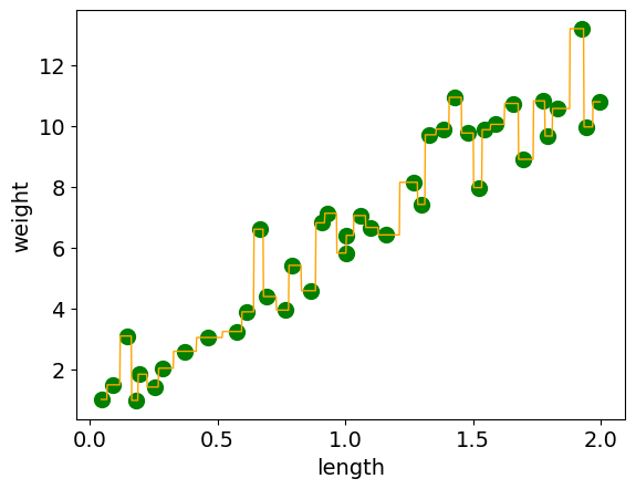
Plotting this we can see our model is trying to get every example correct since n_neighbors=1. (the mean of 1 point is just going to be the point value)

grid = np.linspace(np.min(snake_X_train), np.max(snake_X_train), 1000)
plt.plot(grid, knnr_1.predict(grid[:, np.newaxis]), color='orange', linewidth=1)
plt.scatter(snake_X_train, snake_y_train, color='green', s=100)
plt.xticks(fontsize= 14)
plt.yticks(fontsize= 14)
plt.xlabel("length",fontsize= 14)
plt.ylabel("weight",fontsize= 14)
plt.show()

What happens when we use n_neighbors=10?

knnr_10 = KNeighborsRegressor(n_neighbors=10, weights="uniform")
knnr_10.fit(snake_X_train, snake_y_train)
knnr_10.score(snake_X_train, snake_y_train)

0.9254540554756747

Now we can see we are getting a lower score over the training set. Our score decreased from 1.0 when to had n_neighbors=1 to now having a score of 0.925.

When we plot our model, we can see that it no longer is trying to get every example correct.

grid = np.linspace(np.min(snake_X_train), np.max(snake_X_train), 1000)
plt.plot(grid, knnr_10.predict(grid[:, np.newaxis]), color='orange', linewidth=1)
plt.scatter(snake_X_train, snake_y_train, color='green', s=100)
plt.xticks(fontsize= 14)
plt.yticks(fontsize= 14)
plt.xlabel("length",fontsize= 14)
plt.ylabel("weight",fontsize= 14)
plt.show()

4.4. Pros and Cons of 𝑘 -Nearest Neighbours#

4.4.1. Pros:#

Easy to understand, interpret.
Simply hyperparameter \(k\) (n_neighbors) controlling the fundamental tradeoff.
Can learn very complex functions given enough data.
Lazy learning: Takes no time to fit

4.4.2. Cons:#

Can potentially be VERY slow during prediction time.
Often not that great test accuracy compared to the modern approaches.
Need to scale your features.

4.5. Let’s Practice#

\[\begin{split} X = \begin{bmatrix}5 & 2\\4 & 3\\ 2 & 2\\ 10 & 10\\ 9 & -1\\ 9& 9\end{bmatrix}, \quad y = \begin{bmatrix}0\\0\\1\\1\\1\\2\end{bmatrix}.\end{split}\]

If \(k=3\), what would you predict for \(x=\begin{bmatrix} 0 & 0\end{bmatrix}\) if we were doing regression rather than classification?

Solutions!

1/3 (\(\frac{0 + 0 + 1}{3}\))

4.6. Support Vector Machines (SVMs) with RBF Kernel#

Another popular similarity-based algorithm is Support Vector Machines (SVM).

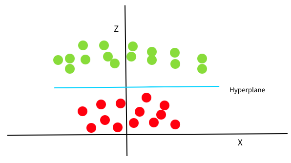
Conceptually, SVMs try to compute which is the best linear decision boundary that can be drawn to separate two (or more) classes. For data in 2D this would be a line, in 3D it would be a plane/surface and so on. A general name for this decision boundary is a hyperplane.

With the training data points below (images in the intro are from this article), there are multiple linear lines/hyperplanes that we could draw that would perfectly separate the points.

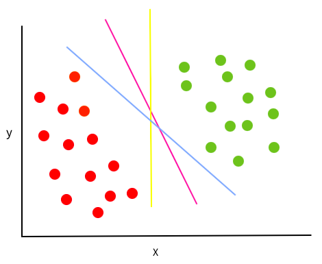
So which one is best? SVMs define “best” as the one with the largest margin to the points from both classes. In other words, the line that are the most in the middle of the border points in each cluster. Since the location of the best margin only depends on the border points from each cluster, these points are called “support points/vectors” (hence the name “support vector machines”).

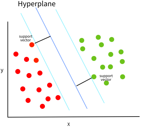
Conceptually it makes sense that the line in the middle of both the clusters is chosen, since we would expect this border to best separate unseen data points. If we instead put the border really close to the green or red cluster, we might make a miss-classification on the new data points if they are not in the exact same spots as the training data. However, we also don’t want one outlier in the training data to completely change the border and we have hyperparameters that can control this as we will see soon.

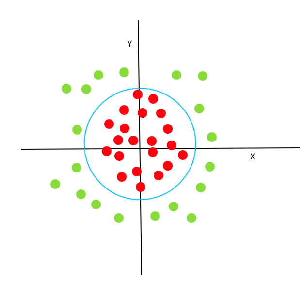
What happens if there is no linear boundary that can be drawn to separate the data as with the points below?

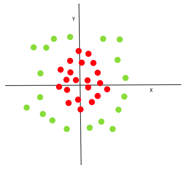
A key concept of SVMs is the transformation of existing dimensions into new ones, where a linear decision boundary can be found. The transformation function is referred to as a kernel, and in this case, we could use a polynomial kernel to create a new dimension such that \(z = x^2 + y^2\). If we plot x (or y) vs z, we can see that there is a linear decision boundary in this new dimension, which perfectly separates the points.

If we transform this decision boundary back to our original xy-space, we can see that it has the shape of a ring. (Here is an animation of this process to help you visualize it).

Kernel transformations allows us to use SVMs on data with complex non-linear decision borders in the original data dimensions. Here, we are going to concentrate on the specific kernel called Radial Basis Functions (RBFs), which is one of the most common and effective kernels and also the default in scikit-learn.

Let’s start by reading in out Canadian and USA cities data yet again.

cities_df = pd.read_csv("data/canada_usa_cities.csv")
cities_train_df, cities_test_df = train_test_split(cities_df, test_size=0.2, random_state=123)
cities_train_df

	longitude	latitude	country
160	-76.4813	44.2307	Canada
127	-81.2496	42.9837	Canada
169	-66.0580	45.2788	Canada
188	-73.2533	45.3057	Canada
187	-67.9245	47.1652	Canada
...	...	...	...
17	-76.3305	44.1255	USA
98	-74.7287	45.0184	Canada
66	-121.4944	38.5816	USA
126	-79.5656	43.6436	Canada
109	-66.9195	44.8938	Canada

167 rows × 3 columns

cities_X_train = cities_train_df.drop(columns=['country'])
cities_y_train = cities_train_df['country']
cities_X_test = cities_test_df.drop(columns=['country'])
cities_y_test = cities_test_df['country']

cities_X_train

	longitude	latitude
160	-76.4813	44.2307
127	-81.2496	42.9837
169	-66.0580	45.2788
188	-73.2533	45.3057
187	-67.9245	47.1652
...	...	...
17	-76.3305	44.1255
98	-74.7287	45.0184
66	-121.4944	38.5816
126	-79.5656	43.6436
109	-66.9195	44.8938

167 rows × 2 columns

cities_y_train

  Canada
  Canada
  Canada
  Canada
  Canada
        ...  
      USA
   Canada
      USA
  Canada
  Canada
Name: country, Length: 167, dtype: object

We can use our training feature table (\(X\)) and target (\(y\)) values by using this new SVM model with (RBF) but with the old set up with .fit() and .score() that we have seen time and time again.

We import the SVC tool from the sklearn.svm library (The “C” in SVC represents Classifier). To import the regressor we import SVR - R for Regressor)

from sklearn.svm import SVC

We can cross-validate and score exactly how we have done it in previous lectures.

svm = SVC()
scores = cross_validate(svm, cities_X_train, cities_y_train, return_train_score=True)
scores_df = pd.DataFrame(scores)
scores_df

	fit_time	score_time	test_score	train_score
0	0.005098	0.001746	0.735294	0.714286
1	0.001753	0.001185	0.705882	0.714286
2	0.001614	0.001279	0.636364	0.761194
3	0.001811	0.001172	0.696970	0.723881
4	0.001568	0.001114	0.696970	0.626866

svm_cv_score = scores_df.mean()
svm_cv_score

fit_time       0.002369
score_time     0.001299
test_score     0.694296
train_score    0.708102
dtype: float64

That validation accuracy does not look too great, let’s have a look at the decision boundary.

svm.fit(cities_X_train, cities_y_train)

mglearn.plots.plot_2d_separator(
        svm, cities_X_train.to_numpy(), fill=True, eps=0.5,alpha=0.4 )
mglearn.discrete_scatter(cities_X_train.iloc[:, 0], cities_X_train.iloc[:, 1], cities_y_train)

[<matplotlib.lines.Line2D at 0x17f39fa00>,
 <matplotlib.lines.Line2D at 0x17f39fca0>]

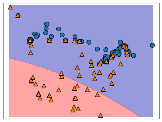
It seems like our model is quite simple, in other words, it is underfitting and not using enough of the specific structure of the training data to draw the decision boundary.

To draw a more specific boundary, we need to tune the SVM hyperparameters.

4.6.1. Hyperparameters of SVM#

There are 2 main hyperparameters for support vector machines with an RBF kernel;

C
gamma

In short, C is the cost/penalty the model accepts for wrongly classified examples in the training data; it trades off correct classification of training examples against maximization of the decision function’s margin. A lower C will reduce the cost/penalty of incorrectly classifying training data, which allows the SVM can be more lenient and draw a simpler decision boundary that likely generalizes better, even if that means getting a few training examples incorrect.

The gamma parameter is specific to the RBF kernel and defines how far the influence of a single training point reaches when constructing the decision boundary. Low values mean ‘far’, creating a simple decision boundary with low curvature (at really low “gamma”, the RBF kernel behaves as a linear SVM kernel). High values mean ‘close’, creating a complex decision boundary with high curvature. Another way of thinking of this is that if you have two dimensional points, and want to construct a third dimension to separate them, gamma controls the shape of the “peaks” when the points are raised. A large gamma gives pointed bumps in the higher dimensions, whereas a small gamma gives a softer, broader bumps.

You can read more in this article and in the scikit-learn’s explanation of RBF SVM parameters.

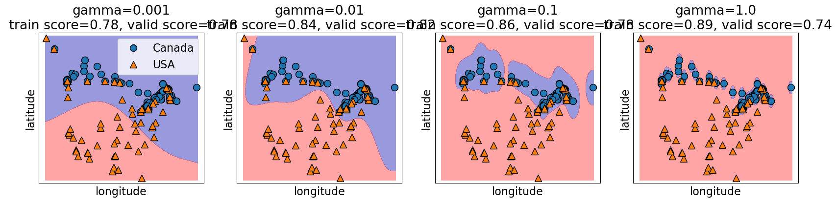
4.6.1.1. `gamma` and the fundamental trade-off#

gamma controls the complexity of a model, just like other hyperparameters we’ve seen.

higher gamma, higher the complexity.
lower gamma, lower the complexity.

gamma = [0.001, 0.01, 0.1, 1.0]
plot_svc_gamma(
    gamma,
    cities_X_train.to_numpy(),
    cities_y_train.to_numpy()
)

4.6.1.2. `C` and the fundamental trade-off#

C also controls the complexity of a model and in turn the fundamental tradeoff.

higher C values, higher the complexity.
lower C values, lower the complexity.

C = [0.1, 10, 1000.0, 100000.0]
plot_svc_C(
    C, cities_X_train.to_numpy(), cities_y_train.to_numpy())

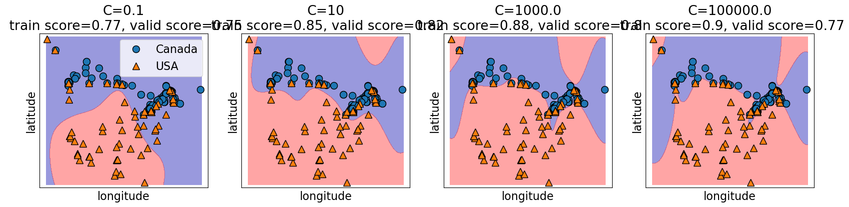
Obtaining optimal validation scores requires a hyperparameter search between both gamma and C to balance the fundamental trade-off. We will learn how to search over multiple hyperparameters at a time in lecture 5.

4.7. Let’s Practice#

True or False

In Scikit Learn’s SVC classifier, large values of gamma tend to result in higher training scores but probably lower validation scores.
If we increase both gamma and C, we can’t be certain if the model becomes more complex or less complex.

Solutions!

True
False

4.8. Let’s Practice - Coding#

Below is some starter code that creates your feature table and target column from the data from the bball.csv dataset (in the data folder).

bball_df = pd.read_csv('data/bball.csv')
bball_df = bball_df[(bball_df['position'] =='G') | (bball_df['position'] =='F')]

# Define X and y
X = bball_df.loc[:, ['height', 'weight', 'salary']]
y = bball_df['position']

Split the dataset into 4 objects: X_train, X_test, y_train, y_test. Make the test set 0.2 (or the train set 0.8) and make sure to use random_state=7.
Create an SVM model with gamma equal to 0.1 and C equal to 10.
Cross-validate using cross_validate() on the objects X_train and y_train specifying the model and making sure to use 5 fold cross-validation and return_train_score=True.
Calculate the mean training and cross-validation scores.

# 1. Split the dataset
X_train, X_test, y_train, y_test = train_test_split(
    X, y, test_size=0.2, random_state=7)

model = SVC(gamma=0.1, C=10)

# 3. Cross-validate
scores_df = pd.DataFrame(cross_validate(model,X_train,y_train, cv=5, return_train_score=True))

scores_df

	fit_time	score_time	test_score	train_score
0	0.003713	0.002048	0.571429	0.994898
1	0.002570	0.001840	0.571429	0.994898
2	0.004793	0.001971	0.551020	0.994898
3	0.002391	0.001668	0.530612	1.000000
4	0.002497	0.001880	0.571429	0.994898

# 4. Calculate the mean training and cross-validation scores.
scores_df.mean()

fit_time       0.003193
score_time     0.001881
test_score     0.559184
train_score    0.995918
dtype: float64

4.9. Preprocessing#

4.9.1. The importance of Preprocessing - An Example of Why#

So far we have seen:

Models: Decision trees, 𝑘-NNs, SVMs with RBF kernel.
Fundamentals: Train-validation-test split, cross-validation, the fundamental tradeoff, the golden rule.

Now …

Preprocessing: Transforming input data into a format a machine learning model can use and understand.

4.9.1.1. Basketball dataset#

Let’s take a look at the bball.csv dataset we just used in practice.

Let’s look at the 3 feature columns height, weight and salary.
Let’s see if these features can help predict the position basketball players is.

bball_df = pd.read_csv('data/bball.csv')
bball_df = bball_df[(bball_df['position'] =='G') | (bball_df['position'] =='F')]
X = bball_df[['weight', 'height', 'salary']]
y =bball_df["position"]
X_train, X_test, y_train, y_test =train_test_split(X, y, test_size=0.20, random_state=123)

X_train

	weight	height	salary
152	79.4	1.88	1588231.0
337	82.1	1.91	2149560.0
130	106.6	2.03	6500000.0
340	106.1	2.08	2961120.0
50	96.2	1.93	4861207.0
...	...	...	...
151	100.7	2.06	4464286.0
120	97.5	1.91	14057730.0
26	96.6	1.93	21000000.0
328	85.7	1.88	15643750.0
139	97.5	2.03	9258000.0

245 rows × 3 columns

y_train

  G
  G
  F
  F
   G
      ..
  F
  G
   G
  G
  F
Name: position, Length: 245, dtype: object

First, let’s see what validations scores we get if we simply predict the most occurring target value in the dataset using the dummy classifier model we saw in the last lecture.

dummy = DummyClassifier(strategy="most_frequent")
scores = cross_validate(dummy, X_train, y_train, return_train_score=True)
print('Mean training score', scores['train_score'].mean().round(2))
print('Mean validation score', scores['test_score'].mean().round(2))

Mean training score 0.57
Mean validation score 0.57

Here we get a mean validation score for our 5 fold cross_validation (5 is the default) of 57%. Let’s now see how much better a \(k\)-nn model does on the data. We saw that it doesn’t do to well on SVM, let’s see if there is a difference with \(k\)-nn.

knn = KNeighborsClassifier()
scores = cross_validate(knn, X_train, y_train, return_train_score=True)
print('Mean training score', scores['train_score'].mean().round(2))
print('Mean validation score', scores['test_score'].mean().round(2))

Mean training score 0.7
Mean validation score 0.5

Ok, not the score we were hoping for.

We are getting a worse score than the dummy classifier. This can’t be right….. and it isn’t and we are going to explain why!

Let’s have a look at just 2 players.

We can see the values in each column.

two_players = X_train.sample(2, random_state=42)
two_players

	weight	height	salary
285	91.2	1.98	1882867.0
236	112.0	2.08	2000000.0

The values in the weight column are around 100.
The values in the height column are around 2.
The values in the salary column are much higher at around 2 million.

Let’s now calculate the distance between the two players.

euclidean_distances(two_players)

array([[     0.        , 117133.00184683],
       [117133.00184683,      0.        ]])

So the distance between the players is 117133.0018.

What happens if we only consider the salary column?

euclidean_distances(two_players[["salary"]])

array([[     0., 117133.],
       [117133.,      0.]])

It looks like it’s almost the same distance!

The distance is completely dominated by the salary column, the feature with the largest values and the weight and height columns are being ignored in the distance calculation.

Does it matter?

Yes! The scale is based on how data was collected.

Features on a smaller scale can be highly informative and there is no good reason to ignore them. We want our model to be robust and not sensitive to the scale.

What about for decision trees? Did scale matter then?

No. In decision trees we ask questions on one feature at a time and so the nodes are created independently without considering others.

We have to scale our columns before we use our \(k\)-nn algorithm (and many others) so they are all using a similar range of values!

And you guessed it - Sklearn has tools called transformers for this.

We’ll be using sklearn’s StandardScaler for this example. We will talk about this type of preprocessing in more detail in a hot minute but for now, concentrate on the syntax.

from sklearn.preprocessing import StandardScaler

scaler = StandardScaler()                    # Create feature transformer object, can accept hyperparameters like models can! 
scaler.fit(X_train)                          # Fitting the transformer on the train split
X_train_scaled = scaler.transform(X_train)   # Transforming the train split
X_test_scaled = scaler.transform(X_test)     # Transforming the test split

sklearn uses fit and transform paradigms for feature transformations. (In model building it was fit and predict or score)

We fit the transformer on the train split and then transform the train split as well as the test split.

pd.DataFrame(X_train_scaled, columns=X_train.columns)

	weight	height	salary
0	-1.552775	-1.236056	-0.728809
1	-1.257147	-0.800950	-0.670086
2	1.425407	0.939473	-0.214967
3	1.370661	1.664650	-0.585185
4	0.286690	-0.510879	-0.386408
...	...	...	...
240	0.779404	1.374579	-0.427932
241	0.429030	-0.800950	0.575680
242	0.330487	-0.510879	1.301942
243	-0.862975	-1.236056	0.741601
244	0.429030	0.939473	0.073560

245 rows × 3 columns

Now if we look at our features they are all within the same scales as opposed to what it was before:

X_train

	weight	height	salary
152	79.4	1.88	1588231.0
337	82.1	1.91	2149560.0
130	106.6	2.03	6500000.0
340	106.1	2.08	2961120.0
50	96.2	1.93	4861207.0
...	...	...	...
151	100.7	2.06	4464286.0
120	97.5	1.91	14057730.0
26	96.6	1.93	21000000.0
328	85.7	1.88	15643750.0
139	97.5	2.03	9258000.0

245 rows × 3 columns

4.9.2. Sklearn’s predict vs transform#

When we make models, we fit and predict(score) with the syntax:

model.fit(X_train, y_train)
X_train_predictions = model.predict(X_train)

With preprocessing, we replace the .predict() step with a .transform() step. We can pass y_train in fit but it’s usually ignored. It allows us to pass it just to be consistent with the usual usage of sklearn’s fit method.

transformer.fit(X_train, [y_train])
X_train_transformed = transformer.transform(X_train)

We can also carry out fitting and transforming in one call using .fit_transform(), but we must be mindful to use it only on the train split and NOT on the test split.

X_train_transformed = transformer.fit_transform(X_train)

Let’s scale our features for this basketball dataset and then compare the results with our original score without scaling.

knn_unscaled = KNeighborsClassifier()
knn_unscaled.fit(X_train, y_train);
print('Train score: ', (knn_unscaled.score(X_train, y_train).round(2)))
print('Test score: ', (knn_unscaled.score(X_test, y_test).round(2)))

Train score:  0.71
Test score:  0.45

knn_scaled = KNeighborsClassifier()
knn_scaled.fit(X_train_scaled, y_train);
print('Train score: ', (knn_scaled.score(X_train_scaled, y_train).round(2)))
print('Test score: ', (knn_scaled.score(X_test_scaled, y_test).round(2)))

Train score:  0.94
Test score:  0.89

The scores with scaled data are now much better compared to the unscaled data in the case of 𝑘-NNs.

We can see now that 𝑘-NN is doing better than the Dummy Classifier when we scaled our features.

We are not carrying out cross-validation here for a reason that we’ll look into soon.

4.9.3. Common preprocessing techniques#

Here are some commonly performed feature transformation techniques we will focus on in this lesson.

Imputation
- Tackling missing values
Scaling
- Scaling of numeric features

4.10. Let’s Practice#

Name a model that will still produce meaningful predictions with different scaled column values.
Complete the following statement with one of the alternatives below: Preprocessing is done ______.
a) To the model but before training
b) To the data before training the model
c) To the model after training
d) To the data after training the model
StandardScaler is a type of what?

True or False

4. Columns with lower magnitudes compared to columns with higher magnitudes are less important when making predictions.
5. A model less sensitive to the scale of the data makes it more robust.

Solutions!

Decision Tree Algorithm
b) To the data before training the model
Transformer
False
True

4.11. California housing data (A case study)#

For the next few examples of preprocessing, we are going to be using a dataset exploring the prices of homes in California to demonstrate feature transformation techniques. The data can be downloaded from this site here. Please make sure that you include it in your data folder that resides in lectures.

This dataset is a modified version of the California Housing dataset available from Luís Torgo’s University of Porto website

The task is to predict median house values in California districts, given several features from these districts.

housing_df = pd.read_csv("data/housing.csv")
train_df, test_df = train_test_split(housing_df, test_size=0.1, random_state=123)

train_df

	longitude	latitude	housing_median_age	total_rooms	total_bedrooms	population	households	median_income	median_house_value	ocean_proximity
6051	-117.75	34.04	22.0	2948.0	636.0	2600.0	602.0	3.1250	113600.0	INLAND
20113	-119.57	37.94	17.0	346.0	130.0	51.0	20.0	3.4861	137500.0	INLAND
14289	-117.13	32.74	46.0	3355.0	768.0	1457.0	708.0	2.6604	170100.0	NEAR OCEAN
13665	-117.31	34.02	18.0	1634.0	274.0	899.0	285.0	5.2139	129300.0	INLAND
14471	-117.23	32.88	18.0	5566.0	1465.0	6303.0	1458.0	1.8580	205000.0	NEAR OCEAN
...	...	...	...	...	...	...	...	...	...	...
7763	-118.10	33.91	36.0	726.0	NaN	490.0	130.0	3.6389	167600.0	<1H OCEAN
15377	-117.24	33.37	14.0	4687.0	793.0	2436.0	779.0	4.5391	180900.0	<1H OCEAN
17730	-121.76	37.33	5.0	4153.0	719.0	2435.0	697.0	5.6306	286200.0	<1H OCEAN
15725	-122.44	37.78	44.0	1545.0	334.0	561.0	326.0	3.8750	412500.0	NEAR BAY
19966	-119.08	36.21	20.0	1911.0	389.0	1241.0	348.0	2.5156	59300.0	INLAND

18576 rows × 10 columns

Some column values are mean/median but some are not.

Before we use this data we need to do some feature engineering.

That means we are going to transform our data into features that may be more meaningful for our prediction.

Let’s add some new features to the dataset which could help predict the target: median_house_value.

train_df = train_df.assign(rooms_per_household = train_df["total_rooms"]/train_df["households"],
                           bedrooms_per_household = train_df["total_bedrooms"]/train_df["households"],
                           population_per_household = train_df["population"]/train_df["households"])

test_df = test_df.assign(rooms_per_household = test_df["total_rooms"]/test_df["households"],
                         bedrooms_per_household = test_df["total_bedrooms"]/test_df["households"],
                         population_per_household = test_df["population"]/test_df["households"])

train_df = train_df.drop(columns=['total_rooms', 'total_bedrooms', 'population'])  
test_df = test_df.drop(columns=['total_rooms', 'total_bedrooms', 'population']) 

train_df

	longitude	latitude	housing_median_age	households	median_income	median_house_value	ocean_proximity	rooms_per_household	bedrooms_per_household	population_per_household
6051	-117.75	34.04	22.0	602.0	3.1250	113600.0	INLAND	4.897010	1.056478	4.318937
20113	-119.57	37.94	17.0	20.0	3.4861	137500.0	INLAND	17.300000	6.500000	2.550000
14289	-117.13	32.74	46.0	708.0	2.6604	170100.0	NEAR OCEAN	4.738701	1.084746	2.057910
13665	-117.31	34.02	18.0	285.0	5.2139	129300.0	INLAND	5.733333	0.961404	3.154386
14471	-117.23	32.88	18.0	1458.0	1.8580	205000.0	NEAR OCEAN	3.817558	1.004801	4.323045
...	...	...	...	...	...	...	...	...	...	...
7763	-118.10	33.91	36.0	130.0	3.6389	167600.0	<1H OCEAN	5.584615	NaN	3.769231
15377	-117.24	33.37	14.0	779.0	4.5391	180900.0	<1H OCEAN	6.016688	1.017972	3.127086
17730	-121.76	37.33	5.0	697.0	5.6306	286200.0	<1H OCEAN	5.958393	1.031564	3.493544
15725	-122.44	37.78	44.0	326.0	3.8750	412500.0	NEAR BAY	4.739264	1.024540	1.720859
19966	-119.08	36.21	20.0	348.0	2.5156	59300.0	INLAND	5.491379	1.117816	3.566092

18576 rows × 10 columns

4.11.1. When is it OK process the data before splitting of the test portion?#

Here it would have been OK to add new features before splitting because we are not using any global information in the data but only looking at one row at a time.
But just to be safe and to avoid accidentally breaking the golden rule, it’s better to do it after splitting.

4.12. Preprocessing: Imputation#

Imputation is handling missing values in our data so let’s explore this a little.

We can .info() we can we all the different column dtypes and also all the number of null values.

train_df.info()

<class 'pandas.core.frame.DataFrame'>
Index: 18576 entries, 6051 to 19966
Data columns (total 10 columns):
 #   Column                    Non-Null Count  Dtype  
---  ------                    --------------  -----  
 0   longitude                 18576 non-null  float64
 1   latitude                  18576 non-null  float64
 2   housing_median_age        18576 non-null  float64
 3   households                18576 non-null  float64
 4   median_income             18576 non-null  float64
 5   median_house_value        18576 non-null  float64
 6   ocean_proximity           18576 non-null  object 
 7   rooms_per_household       18576 non-null  float64
 8   bedrooms_per_household    18391 non-null  float64
 9   population_per_household  18576 non-null  float64
dtypes: float64(9), object(1)
memory usage: 1.6+ MB

We see that we have all columns with dtype float64 except for ocean_proximity which appears categorical.

We also notice that the bedrooms_per_household column appears to have some Non-Null rows (ie missing values).

train_df["bedrooms_per_household"].isnull().sum()

Knowing this information let’s build a model.

When we create our feature table and target objects, we are going to drop the categorical variable ocean_proximity. Currently, we don’t know how to build models with categorical data, but we will shortly. We will return to this column soon.

X_train = train_df.drop(columns=["median_house_value", "ocean_proximity"])
y_train = train_df["median_house_value"]

X_test = test_df.drop(columns=["median_house_value", "ocean_proximity"])
y_test = test_df["median_house_value"]

knn = KNeighborsRegressor()

What happens when we try to fit our model with this data?

knn.fit(X_train, y_train)

---------------------------------------------------------------------------
ValueError                                Traceback (most recent call last)
Cell In[45], line 1
----> 1 knn.fit(X_train, y_train)

File ~/opt/miniconda3/envs/571/lib/python3.10/site-packages/sklearn/base.py:1152, in _fit_context.<locals>.decorator.<locals>.wrapper(estimator, *args, **kwargs)
   estimator._validate_params()
with config_context(
   skip_parameter_validation=(
       prefer_skip_nested_validation or global_skip_validation
   )
):
-> 1152     return fit_method(estimator, *args, **kwargs)

File ~/opt/miniconda3/envs/571/lib/python3.10/site-packages/sklearn/neighbors/_regression.py:218, in KNeighborsRegressor.fit(self, X, y)
@_fit_context(
   # KNeighborsRegressor.metric is not validated yet
   prefer_skip_nested_validation=False
)
def fit(self, X, y):
   """Fit the k-nearest neighbors regressor from the training dataset.

   Parameters
   (...)
       The fitted k-nearest neighbors regressor.
   """
--> 218     return self._fit(X, y)

File ~/opt/miniconda3/envs/571/lib/python3.10/site-packages/sklearn/neighbors/_base.py:456, in NeighborsBase._fit(self, X, y)
if self._get_tags()["requires_y"]:
   if not isinstance(X, (KDTree, BallTree, NeighborsBase)):
--> 456         X, y = self._validate_data(
           X, y, accept_sparse="csr", multi_output=True, order="C"
       )
   if is_classifier(self):
       # Classification targets require a specific format
       if y.ndim == 1 or y.ndim == 2 and y.shape[1] == 1:

File ~/opt/miniconda3/envs/571/lib/python3.10/site-packages/sklearn/base.py:622, in BaseEstimator._validate_data(self, X, y, reset, validate_separately, cast_to_ndarray, **check_params)
       y = check_array(y, input_name="y", **check_y_params)
   else:
--> 622         X, y = check_X_y(X, y, **check_params)
   out = X, y
if not no_val_X and check_params.get("ensure_2d", True):

File ~/opt/miniconda3/envs/571/lib/python3.10/site-packages/sklearn/utils/validation.py:1146, in check_X_y(X, y, accept_sparse, accept_large_sparse, dtype, order, copy, force_all_finite, ensure_2d, allow_nd, multi_output, ensure_min_samples, ensure_min_features, y_numeric, estimator)
       estimator_name = _check_estimator_name(estimator)
   raise ValueError(
       f"{estimator_name} requires y to be passed, but the target y is None"
   )
-> 1146 X = check_array(
   X,
   accept_sparse=accept_sparse,
   accept_large_sparse=accept_large_sparse,
   dtype=dtype,
   order=order,
   copy=copy,
   force_all_finite=force_all_finite,
   ensure_2d=ensure_2d,
   allow_nd=allow_nd,
   ensure_min_samples=ensure_min_samples,
   ensure_min_features=ensure_min_features,
   estimator=estimator,
   input_name="X",
)
y = _check_y(y, multi_output=multi_output, y_numeric=y_numeric, estimator=estimator)
check_consistent_length(X, y)

File ~/opt/miniconda3/envs/571/lib/python3.10/site-packages/sklearn/utils/validation.py:957, in check_array(array, accept_sparse, accept_large_sparse, dtype, order, copy, force_all_finite, ensure_2d, allow_nd, ensure_min_samples, ensure_min_features, estimator, input_name)
       raise ValueError(
           "Found array with dim %d. %s expected <= 2."
           % (array.ndim, estimator_name)
       )
   if force_all_finite:
--> 957         _assert_all_finite(
           array,
           input_name=input_name,
           estimator_name=estimator_name,
           allow_nan=force_all_finite == "allow-nan",
       )
if ensure_min_samples > 0:
   n_samples = _num_samples(array)

File ~/opt/miniconda3/envs/571/lib/python3.10/site-packages/sklearn/utils/validation.py:122, in _assert_all_finite(X, allow_nan, msg_dtype, estimator_name, input_name)
if first_pass_isfinite:
   return
--> 122 _assert_all_finite_element_wise(
   X,
   xp=xp,
   allow_nan=allow_nan,
   msg_dtype=msg_dtype,
   estimator_name=estimator_name,
   input_name=input_name,
)

File ~/opt/miniconda3/envs/571/lib/python3.10/site-packages/sklearn/utils/validation.py:171, in _assert_all_finite_element_wise(X, xp, allow_nan, msg_dtype, estimator_name, input_name)
if estimator_name and input_name == "X" and has_nan_error:
   # Improve the error message on how to handle missing values in
   # scikit-learn.
   msg_err += (
       f"\n{estimator_name} does not accept missing values"
       " encoded as NaN natively. For supervised learning, you might want"
   (...)
       "#estimators-that-handle-nan-values"
   )
--> 171 raise ValueError(msg_err)

ValueError: Input X contains NaN.
KNeighborsRegressor does not accept missing values encoded as NaN natively. For supervised learning, you might want to consider sklearn.ensemble.HistGradientBoostingClassifier and Regressor which accept missing values encoded as NaNs natively. Alternatively, it is possible to preprocess the data, for instance by using an imputer transformer in a pipeline or drop samples with missing values. See https://scikit-learn.org/stable/modules/impute.html You can find a list of all estimators that handle NaN values at the following page: https://scikit-learn.org/stable/modules/impute.html#estimators-that-handle-nan-values

Input contains NaN, infinity or a value too large for dtype('float64').

The classifier can’t deal with missing values (NaNs).

How can we deal with this problem?

4.12.1. Why we don’t drop the rows#

We could drop any rows that are missing information but that’s problematic too.

Then we would need to do the same in our test set.

And what happens if we get missing values in our deployment data? what then?

Furthermore, what if the missing values don’t occur at random and we’re systematically dropping certain data? Perhaps a certain type of house contributes to more missing values.

Dropping the rows is not a great solution, especially if there’s a lot of missing values.

X_train.shape

(18576, 8)

X_train_no_nan = X_train.dropna()
X_train_no_nan.shape

(18391, 8)

4.12.2. Why we don’t drop the column#

If we drop the column instead of the rows, we are throwing away, in this case, 18391 values just because we don’t have 185 missing values out of a total of 18567.

We are throwing away 99% of the column’s data because we are missing 1%.

But perhaps if we were missing 99.9% of the column values, for example, it would make more sense to drop the column.

X_train.shape

(18576, 8)

X_train_no_col = X_train.dropna(axis=1)
X_train_no_col.shape

(18576, 7)

4.12.3. Why we use imputation#

With Imputation, we invent values for the missing data.

Using sklearn’s transformer SimpleImputer, we can impute the NaN values in the data with some value.

from sklearn.impute import SimpleImputer

We can impute missing values in:

Categorical columns:
- with the most frequent value
- with a constant of our choosing.
Numeric columns:
- with the mean of the column
- with the median of the column
- or a constant of our choosing.

If I sort the values by bedrooms_per_household and look at the end of the dataframe, we can see our missing values in the bedrooms_per_household column.

Pay close attention to index 7763 since we are going to look at this row after imputation.

X_train.sort_values('bedrooms_per_household').tail(10)

	longitude	latitude	housing_median_age	households	median_income	rooms_per_household	bedrooms_per_household	population_per_household
18786	-122.42	40.44	16.0	181.0	2.1875	5.491713	NaN	2.734807
17923	-121.97	37.35	30.0	386.0	4.6328	5.064767	NaN	2.588083
16880	-122.39	37.59	32.0	715.0	6.1323	6.289510	NaN	2.581818
4309	-118.32	34.09	44.0	726.0	1.6760	3.672176	NaN	3.163912
538	-122.28	37.78	29.0	1273.0	2.5762	4.048704	NaN	2.938727
4591	-118.28	34.06	42.0	1179.0	1.2254	2.096692	NaN	3.218830
19485	-120.98	37.66	10.0	255.0	0.9336	3.662745	NaN	1.572549
6962	-118.05	33.99	38.0	357.0	3.7328	4.535014	NaN	2.481793
14970	-117.01	32.74	31.0	677.0	2.6973	5.129985	NaN	3.098966
7763	-118.10	33.91	36.0	130.0	3.6389	5.584615	NaN	3.769231

Using the same fit and transform syntax we saw earlier for transformers, we can impute the NaN values.

Here we specify strategy="median" which replaces all the missing values with the column median.

We fit on the training data and transform it on the train and test splits.

imputer = SimpleImputer(strategy="median")
imputer.fit(X_train);
X_train_imp = imputer.transform(X_train)
X_test_imp = imputer.transform(X_test)

X_train_imp

array([[-117.75      ,   34.04      ,   22.        , ...,    4.89700997,
           1.05647841,    4.31893688],
       [-119.57      ,   37.94      ,   17.        , ...,   17.3       ,
           6.5       ,    2.55      ],
       [-117.13      ,   32.74      ,   46.        , ...,    4.73870056,
           1.08474576,    2.0579096 ],
       ...,
       [-121.76      ,   37.33      ,    5.        , ...,    5.95839311,
           1.03156385,    3.49354376],
       [-122.44      ,   37.78      ,   44.        , ...,    4.7392638 ,
           1.02453988,    1.7208589 ],
       [-119.08      ,   36.21      ,   20.        , ...,    5.49137931,
           1.11781609,    3.56609195]])

Ok, the output of this isn’t a dataframe but a NumPy array!

I can do a bit of wrangling here to take a look at this new array with our previous column labels and as a dataframe.

If I search for our index 7763 which previously contained a NaN value, we can see that now I have the median value for the bedrooms_per_household column from the X_train dataframe.

X_train_imp_df = pd.DataFrame(X_train_imp, columns = X_train.columns, index = X_train.index)
X_train_imp_df.loc[[7763]]

	longitude	latitude	housing_median_age	households	median_income	rooms_per_household	bedrooms_per_household	population_per_household
7763	-118.1	33.91	36.0	130.0	3.6389	5.584615	1.04886	3.769231

X_train['bedrooms_per_household'].median()

1.0488599348534202

X_train_imp_df.loc[[7763]]

	longitude	latitude	housing_median_age	households	median_income	rooms_per_household	bedrooms_per_household	population_per_household
7763	-118.1	33.91	36.0	130.0	3.6389	5.584615	1.04886	3.769231

Now when we try and fit our model using X_train_imp, it works!

knn = KNeighborsRegressor()
knn.fit(X_train_imp, y_train)
knn.score(X_train_imp, y_train)

0.5609808539232339

4.12.4. More sophisticated imputation methods#

Instead of using the most frequent label or an average of all the data when we impute, we can try to use ML-techniques also for the imputation step. For example, we can use an average value from the rows that are the most similar to observation that have a missing value, by first running a similarity ML-method such as kNN to determine which these rows are (but note that this is still sensitive to rescaling of the data). Instead of subsetting the data we can also use different regression methods to build a function that uses all the existing features to predicted what the value of the missing feature should be. These methods generally perform better than simple imputation that we use here, but they also require more careful implementation and higher computational cost. You can read more about them in these links:

https://scikit-learn.org/stable/modules/impute.html
https://scikit-learn.org/stable/auto_examples/impute/plot_iterative_imputer_variants_comparison.html#sphx-glr-auto-examples-impute-plot-iterative-imputer-variants-comparison-py
https://towardsdatascience.com/6-different-ways-to-compensate-for-missing-values-data-imputation-with-examples-6022d9ca0779

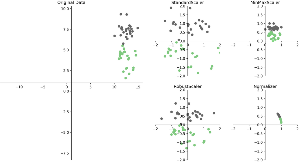
4.13. Preprocessing: Scaling#

So we’ve seen why scaling is important earlier but let’s take a little bit of a closer look here. There are many ways to scale your data but we are going to look at 2 of them.

Approach	What it does	How to update \(X\) (but see below!)	sklearn implementation
normalization	sets range to \([0,1]\)	`X -= np.min(X,axis=0)` `X /= np.max(X,axis=0)`	`MinMaxScaler()`
standardization	sets sample mean to \(0\), s.d. to \(1\)	`X -= np.mean(X,axis=0)` `X /= np.std(X,axis=0)`	`StandardScaler()`

For more resources and articles on this, see here and here.

Let’s see what happens when we use each of them.

from sklearn.preprocessing import MinMaxScaler, StandardScaler

First, let’s see how standardization is done first.

scaler = StandardScaler()
X_train_scaled_std = scaler.fit_transform(X_train_imp)
X_test_scaled_std = scaler.transform(X_test_imp)
pd.DataFrame(X_train_scaled_std, columns=X_train.columns, index=X_train.index)

	longitude	latitude	housing_median_age	households	median_income	rooms_per_household	bedrooms_per_household	population_per_household
6051	0.908140	-0.743917	-0.526078	0.266135	-0.389736	-0.210591	-0.083813	0.126398
20113	-0.002057	1.083123	-0.923283	-1.253312	-0.198924	4.726412	11.166631	-0.050132
14289	1.218207	-1.352930	1.380504	0.542873	-0.635239	-0.273606	-0.025391	-0.099240
13665	1.128188	-0.753286	-0.843842	-0.561467	0.714077	0.122307	-0.280310	0.010183
14471	1.168196	-1.287344	-0.843842	2.500924	-1.059242	-0.640266	-0.190617	0.126808
...	...	...	...	...	...	...	...	...
7763	0.733102	-0.804818	0.586095	-0.966131	-0.118182	0.063110	-0.099558	0.071541
15377	1.163195	-1.057793	-1.161606	0.728235	0.357500	0.235096	-0.163397	0.007458
17730	-1.097293	0.797355	-1.876574	0.514155	0.934269	0.211892	-0.135305	0.044029
15725	-1.437367	1.008167	1.221622	-0.454427	0.006578	-0.273382	-0.149822	-0.132875
19966	0.242996	0.272667	-0.684960	-0.396991	-0.711754	0.025998	0.042957	0.051269

18576 rows × 8 columns

Here, any negative values represent values that are lower than the calculated feature mean and anything positive and greater than 0 are values greater than the original column mean.

knn = KNeighborsRegressor()
knn.fit(X_train_imp, y_train);
print('Unscaled training score :', knn.score(X_train_imp, y_train).round(3))

Unscaled training score : 0.561

knn = KNeighborsRegressor()
knn.fit(X_train_scaled_std, y_train)
print('Scaled training score :', knn.score(X_train_scaled_std, y_train))

Scaled training score : 0.7978563117812038

scaler = MinMaxScaler()
X_train_scaled_norm = scaler.fit_transform(X_train_imp)
X_test_scaled_norm = scaler.transform(X_test_imp)
pd.DataFrame(X_train_scaled_norm, columns=X_train.columns, index=X_train.index).head()

	longitude	latitude	housing_median_age	households	median_income	rooms_per_household	bedrooms_per_household	population_per_household
6051	0.657371	0.159405	0.411765	0.098832	0.181039	0.028717	0.021437	0.002918
20113	0.476096	0.573858	0.313725	0.003124	0.205942	0.116642	0.182806	0.001495
14289	0.719124	0.021254	0.882353	0.116264	0.148998	0.027594	0.022275	0.001099
13665	0.701195	0.157279	0.333333	0.046703	0.325099	0.034645	0.018619	0.001981
14471	0.709163	0.036132	0.333333	0.239599	0.093661	0.021064	0.019905	0.002922

Looking at the data after normalizing it, we see this time there are no negative values and they all are between 0 and 1.

And the score now?

knn = KNeighborsRegressor()
knn.fit(X_train_scaled_norm, y_train)
print('Scaled training score :',knn.score(X_train_scaled_norm, y_train))

Scaled training score : 0.8006485189373813

Big difference in the KNN training performance after scaling the data.
But we saw last week that the training score doesn’t tell us much. We should look at the cross-validation score.

So let’s see how we can do this but first…. let’s practice!

4.14. Let’s Practice#

1. When/Why do we need to impute our data?
2. If we have NaN values in our data, can we simply drop the column missing the data?
3. Which scaling method will never produce negative values?
4. Which scaling method will never produce values greater than 1?
5. Which scaling method will produce values where the range depends on the values in the data?

True or False

6. SimpleImputer is a type of transformer.
7. Scaling is a form of transformation.
8. We can use SimpleImputer to impute values that are missing from numerical and categorical columns.

Solutions!

When we have missing data so that sklearn doesn’t give an error.
No but we can if the majority of the values are missing from the column.
Normalization (MinMaxScaler)
Normalization (MinMaxScaler)
Standardization (StandardScaler)
True
True
True

4.15. Feature transformations and the golden rule#

How to carry out cross-validation?

Last week we saw that cross-validation is a better way to get a realistic assessment of the model.
Let’s try cross-validation with transformed data.

knn = KNeighborsRegressor()
scores = cross_validate(knn, X_train_scaled_std, y_train, return_train_score=True)
pd.DataFrame(scores)

	fit_time	score_time	test_score	train_score
0	0.009116	0.160559	0.696373	0.794236
1	0.008147	0.134536	0.684447	0.791467
2	0.007982	0.143678	0.695532	0.789436
3	0.007958	0.144992	0.679478	0.793243
4	0.008038	0.089106	0.680657	0.794820

Do you see any problem here?

We are using our X_train_scaled in our cross_validate() function which already has all our preprocessing done.

That means that our validation set information is being used to calculate the mean and standard deviation (or min and max values for MinMaxScaler) for our training split!

We are allowing information from the validation set to leak into the training step.

What was our golden rule of machine learning again? Oh yeah -> Our test data should not influence our training data.

This applies also to our validation data and that it also should not influence our training data.

With imputation and scaling, we are scaling and imputing values based on all the information in the data meaning the training data AND the validation data and so we are not adhering to the golden rule anymore.

Every row in our x_train_scaled has now been influenced in a minor way by every other row in x_train_scaled.

With scaling every row has been transformed based on all the data before splitting between training and validation.

We need to take care that we are keeping our validation data truly as unseen data.

Before we look at the right approach to this, let’s look at the WRONG approaches.

4.15.1. Bad methodology 1: Scaling the data separately#

We make our transformer, we fit it on the training data and then transform the training data.

Then, we make a second transformer, fit it on the test data and then transform our test data.

scaler = StandardScaler();
scaler.fit(X_train_imp);
X_train_scaled = scaler.transform(X_train_imp)


# Creating a separate object for scaling test data - Not a good idea.
scaler = StandardScaler();
scaler.fit(X_test_imp); # Calling fit on the test data - Yikes! 
X_test_scaled = scaler.transform(X_test_imp) # Transforming the test data using the scaler fit on test data ... Bad! 


knn = KNeighborsRegressor()
knn.fit(X_train_scaled, y_train);
print("Training score: ", knn.score(X_train_scaled, y_train).round(2))
print("Test score: ", knn.score(X_test_scaled, y_test).round(2))

Training score:  0.8
Test score:  0.7

This is bad because we are using two different StandardScaler objects but we want to apply the same transformation on the training and test splits.

The test data will have different values than the training data producing a different transformation than the training data.

We should never fit on test data, whether it’s to build a model or with a transforming, test data should never be exposed to the fit function.

4.15.2. Bad methodology 2: Scaling the data together#

The next mistake is when we scale the data together. So instead of splitting our data, we are combining our training and testing and scaling it together.

X_train_imp.shape, X_test_imp.shape

((18576, 8), (2064, 8))

# join the train and test sets back together
XX = np.vstack((X_train_imp, X_test_imp))## Don't do it! 
XX.shape 

(20640, 8)

scaler = StandardScaler()
scaler.fit(XX)
XX_scaled = scaler.transform(XX) 
XX_train = XX_scaled[:18576]
XX_test = XX_scaled[18576:]

knn = KNeighborsRegressor()
knn.fit(XX_train, y_train);
print('Train score: ', (knn.score(XX_train, y_train).round(2))) # Misleading score
print('Test score: ', (knn.score(XX_test, y_test).round(2))) # Misleading score

Train score:  0.8
Test score:  0.71

Here we are scaling the train and test splits together.

The golden rule says that the test data shouldn’t influence the training in any way.

Information from the test split is now affecting the mean for standardization!

This is a clear violation of the golden rule.

So what do we do? Enter ….

4.16. Pipelines#

Scikit-learn Pipeline is here to save the day!

A pipeline is a sklearn function that contains a sequence of steps.

Essentially we give it all the actions we want to do with our data such as transformers and models and the pipeline will execute them in steps.

from sklearn.pipeline import Pipeline

Let’s combine the preprocessing and model with pipeline.

we will instruct the pipeline to:

Do imputation using SimpleImputer() using a strategy of “median”
Scale our data using StandardScaler
Build a KNeighborsRegressor.

(The last step should be a model and earlier steps should be transformers)

Note: The input for Pipeline is a list containing tuples (one for each step).

pipe = Pipeline([
        ("imputer", SimpleImputer(strategy="median")),
        ("scaler", StandardScaler()),
        ("reg", KNeighborsRegressor())
])

pipe.fit(X_train, y_train)

Pipeline(steps=[('imputer', SimpleImputer(strategy='median')),
                ('scaler', StandardScaler()), ('reg', KNeighborsRegressor())])

In a Jupyter environment, please rerun this cell to show the HTML representation or trust the notebook.
On GitHub, the HTML representation is unable to render, please try loading this page with nbviewer.org.

Note that we are passing X_train and NOT the imputed or scaled data here.

When we call fit the pipeline is carrying out the following steps:

Fit SimpleImputer on X_train.
Transform X_train using the fit SimpleImputer to create X_train_imp.
Fit StandardScaler on X_train_imp.
Transform X_train_imp using the fit StandardScaler to create X_train_imp_scaled.
Fit the model (KNeighborsRegressor in our case) on X_train_imp_scaled.

pipe.predict(X_train)

array([126500., 117380., 187700., ..., 259500., 308120.,  60860.])

When we call predict on our data, the following steps are carrying out:

Transform X_train using the fit SimpleImputer to create X_train_imp.
Transform X_train_imp using the fit StandardScaler to create X_train_imp_scaled.
Predict using the fit model (KNeighborsRegressor in our case) on X_train_imp_scaled.

It is not fitting any of the data this time.

https://amueller.github.io/COMS4995-s20/slides/aml-04-preprocessing/images/pipeline.png

Source

We can’t accidentally re-fit the preprocessor on the test data as we did before.

It automatically makes sure the same transformations are applied to train and test.

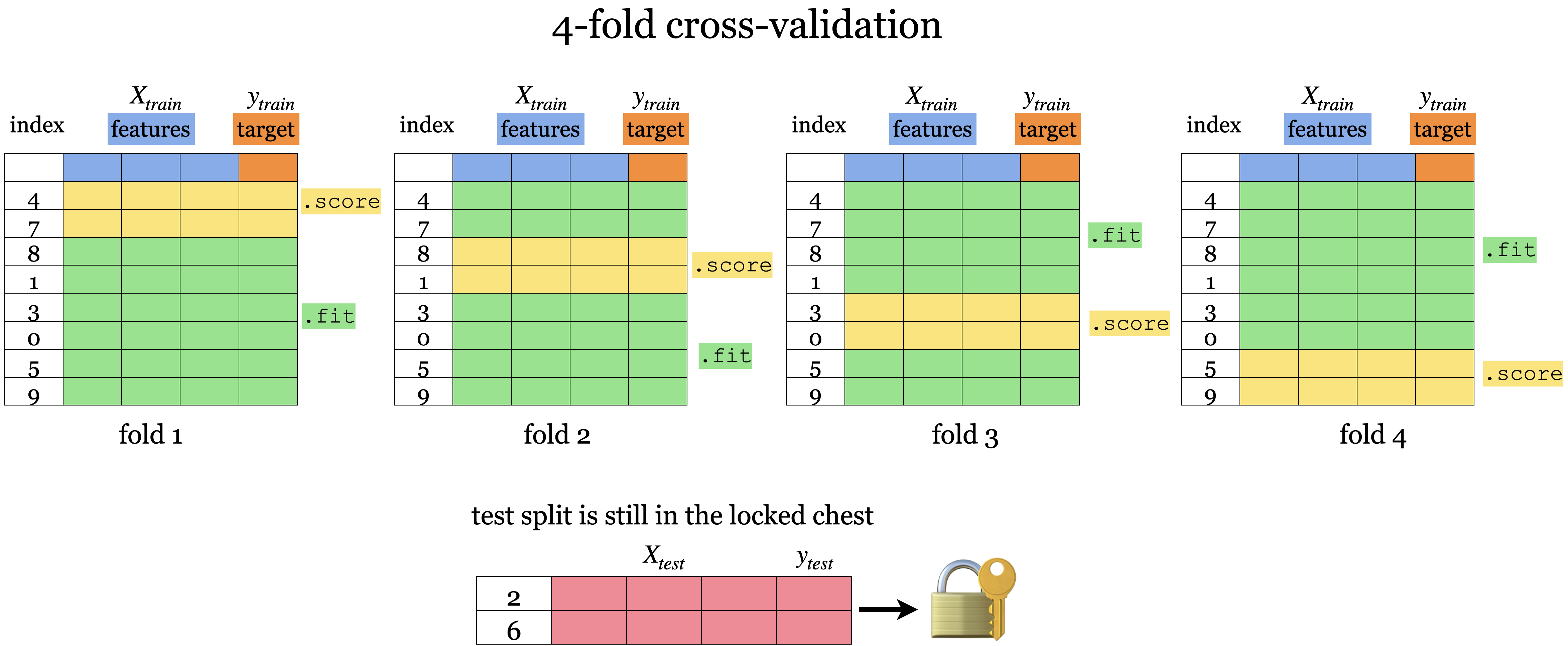
Now when we do cross-validation on the pipeline the transformers and the model are refit on each fold.

The pipeline applies the fit_transform on the train portion of the data and only transform on the validation portion in each fold.

This is how to avoid the Golden Rule violation!

scores_processed = cross_validate(pipe, X_train, y_train, return_train_score=True)
pd.DataFrame(scores_processed)

	fit_time	score_time	test_score	train_score
0	0.022580	0.157835	0.693883	0.792395
1	0.020257	0.140336	0.685017	0.789108
2	0.019219	0.143953	0.694409	0.787796
3	0.019068	0.147445	0.677055	0.792444
4	0.019125	0.117869	0.714494	0.823421

pd.DataFrame(scores_processed).mean()

fit_time       0.020050
score_time     0.141488
test_score     0.692972
train_score    0.797033
dtype: float64

dummy = DummyRegressor()
scores = cross_validate(dummy, X_train, y_train, return_train_score=True)
pd.DataFrame(scores).mean()

fit_time       0.001078
score_time     0.000348
test_score    -0.000838
train_score    0.000000
dtype: float64

We can trust here now that the scores are not influenced but the training data and all our steps were done efficiently and easily too.

4.17. Let’s Practice#

1. Which of the following steps cannot be used in a pipeline?

a) Scaling
b) Model building
c) Imputation
d) Data Splitting

2. Why can’t we fit and transform the training and test data together?

True or False

3. We have to be careful of the order we put each transformation and model in a pipeline.
4. Pipelines will fit and transform on both the training and validation folds during cross-validation.

Solutions!

Data Splitting
It’s violating the golden rule of keeping the test data separate.
True
False

4.18. Let’s Practice - Coding#

Let’s bring in the basketball dataset again.

# Loading in the data
bball_df = pd.read_csv('data/bball.csv')
bball_df = bball_df[(bball_df['position'] =='G') | (bball_df['position'] =='F')]

# Define X and y
X = bball_df.loc[:, ['height', 'weight', 'salary']]
y = bball_df['position']

# Split the dataset
X_train, X_test, y_train, y_test = train_test_split(
    X, y, test_size=0.2, random_state=7)

Build a pipeline named bb_pipe that:
1. Imputes using “mean” as a strategy,
2. scale using MinMaxScaler
3. builds a KNeighborsClassifier.
Next, do 5 fold cross-validation on the pipeline using X_train and y_train and save the results in a dataframe. Take the mean of each column and assess your model.

Solutions

1.

pipe = Pipeline([
        ("imputer", SimpleImputer(strategy="mean")),
        ("scaler", MinMaxScaler()),
        ("reg", KNeighborsClassifier())
])

2.

pd.DataFrame(cross_validate(pipe, X_train, y_train, return_train_score=True)).mean()

fit_time       0.002501
score_time     0.003170
test_score     0.873469
train_score    0.916327
dtype: float64

4.19. What We’ve Learned Today #

How the \(k\)NN algorithm works for regression.
How to build an SVM with RBF kernel model.
How changing gamma and C hyperparameters affects the fundamental tradeoff.
How to imputer values when we are missing data.
Why it’s important to scale our features.
How to scales our features.
How to build a pipeline that executes a number of steps without breaking the golden rule of ML.

BAIT 509
Business Applications of Machine Learning

kNN regression, Support Vector Machines, and Feature Preprocessing

Contents

4. kNN regression, Support Vector Machines, and Feature Preprocessing#

4.1. Lecture Learning Objectives#

4.2. Five Minute Recap/ Lightning Questions#

4.2.1. Some lingering questions#

4.3. Regression with \(k\)-NN#

4.4. Pros and Cons of 𝑘 -Nearest Neighbours#

4.4.1. Pros:#

4.4.2. Cons:#

4.5. Let’s Practice#

4.6. Support Vector Machines (SVMs) with RBF Kernel#

4.6.1. Hyperparameters of SVM#

4.6.1.1. `gamma` and the fundamental trade-off#

4.6.1.2. `C` and the fundamental trade-off#

4.7. Let’s Practice#

4.8. Let’s Practice - Coding#

4.9. Preprocessing#

4.9.1. The importance of Preprocessing - An Example of Why#

4.9.1.1. Basketball dataset#

4.9.2. Sklearn’s predict vs transform#

4.9.3. Common preprocessing techniques#

4.10. Let’s Practice#

4.11. California housing data (A case study)#

4.11.1. When is it OK process the data before splitting of the test portion?#

4.12. Preprocessing: Imputation#

4.12.1. Why we don’t drop the rows#

4.12.2. Why we don’t drop the column#

4.12.3. Why we use imputation#

4.12.4. More sophisticated imputation methods#

4.13. Preprocessing: Scaling#

4.14. Let’s Practice#

4.15. Feature transformations and the golden rule#

4.15.1. Bad methodology 1: Scaling the data separately#

4.15.2. Bad methodology 2: Scaling the data together#

4.16. Pipelines#

4.17. Let’s Practice#

4.18. Let’s Practice - Coding#

4.19. What We’ve Learned Today #

BAIT 509Business Applications of Machine Learning

kNN regression, Support Vector Machines, and Feature Preprocessing

Contents

4. kNN regression, Support Vector Machines, and Feature Preprocessing#

4.1. Lecture Learning Objectives#

4.2. Five Minute Recap/ Lightning Questions#

4.2.1. Some lingering questions#

4.3. Regression with \(k\)-NN#

4.4. Pros and Cons of 𝑘 -Nearest Neighbours#

4.4.1. Pros:#

4.4.2. Cons:#

4.5. Let’s Practice#

4.6. Support Vector Machines (SVMs) with RBF Kernel#

4.6.1. Hyperparameters of SVM#

4.6.1.1. gamma and the fundamental trade-off#

4.6.1.2. C and the fundamental trade-off#

4.7. Let’s Practice#

4.8. Let’s Practice - Coding#

4.9. Preprocessing#

4.9.1. The importance of Preprocessing - An Example of Why#

4.9.1.1. Basketball dataset#

4.9.2. Sklearn’s predict vs transform#

4.9.3. Common preprocessing techniques#

4.10. Let’s Practice#

4.11. California housing data (A case study)#

4.11.1. When is it OK process the data before splitting of the test portion?#

4.12. Preprocessing: Imputation#

4.12.1. Why we don’t drop the rows#

4.12.2. Why we don’t drop the column#

4.12.3. Why we use imputation#

4.12.4. More sophisticated imputation methods#

4.13. Preprocessing: Scaling#

4.14. Let’s Practice#

4.15. Feature transformations and the golden rule#

4.15.1. Bad methodology 1: Scaling the data separately#

4.15.2. Bad methodology 2: Scaling the data together#

4.16. Pipelines#

4.17. Let’s Practice#

4.18. Let’s Practice - Coding#

4.19. What We’ve Learned Today#

BAIT 509
Business Applications of Machine Learning

4.6.1.1. `gamma` and the fundamental trade-off#

4.6.1.2. `C` and the fundamental trade-off#

4.19. What We’ve Learned Today #