Preprocessing Categorical Features and Column Transformer
Contents
5. Preprocessing Categorical Features and Column Transformer#
5.1. Lecture Learning Objectives#
Identify when it’s appropriate to apply ordinal encoding vs one-hot encoding.
Explain strategies to deal with categorical variables with too many categories.
Explain
handle_unknown="ignore"hyperparameter ofscikit-learn’sOneHotEncoder.Use the scikit-learn
ColumnTransformerfunction to implement preprocessing functions such asMinMaxScalerandOneHotEncoderto numeric and categorical features simultaneously.Use
ColumnTransformerto build all our transformations together into one object and use it withscikit-learnpipelines.Explain why text data needs a different treatment than categorical variables.
Use
scikit-learn’sCountVectorizerto encode text data.Explain different hyperparameters of
CountVectorizer.
5.2. Five Minute Recap/ Lightning Questions#
Where does most of the work happen in \(k\)-nn -
fitorpredict?What are the 2 hyperparameters we looked at with Support Vector Machines with RBF kernel?
What is the range of values after Normalization?
Imputation will help data with missing values by removing which of the following; the column, the row or neither?
Pipelines help us not violate what?
5.2.1. Some lingering questions#
What about categorical features??! How do we use them in our model!?
How do we combine everything?!
What about data with text?
5.3. Introducing Categorical Feature Preprocessing#
Let’s bring back our California housing dataset that we explored last class. Remember we engineered some of the features in the data.
import pandas as pd
from sklearn.model_selection import train_test_split


housing_df = pd.read_csv("data/housing.csv")
train_df, test_df = train_test_split(housing_df, test_size=0.1, random_state=123)

train_df = train_df.assign(rooms_per_household = train_df["total_rooms"]/train_df["households"],
                           bedrooms_per_household = train_df["total_bedrooms"]/train_df["households"],
                           population_per_household = train_df["population"]/train_df["households"])

test_df = test_df.assign(rooms_per_household = test_df["total_rooms"]/test_df["households"],
                         bedrooms_per_household = test_df["total_bedrooms"]/test_df["households"],
                         population_per_household = test_df["population"]/test_df["households"])

train_df = train_df.drop(columns=['total_rooms', 'total_bedrooms', 'population'])
test_df = test_df.drop(columns=['total_rooms', 'total_bedrooms', 'population'])

train_df
| longitude | latitude | housing_median_age | households | median_income | median_house_value | ocean_proximity | rooms_per_household | bedrooms_per_household | population_per_household | |
|---|---|---|---|---|---|---|---|---|---|---|
| 6051 | -117.75 | 34.04 | 22.0 | 602.0 | 3.1250 | 113600.0 | INLAND | 4.897010 | 1.056478 | 4.318937 |
| 20113 | -119.57 | 37.94 | 17.0 | 20.0 | 3.4861 | 137500.0 | INLAND | 17.300000 | 6.500000 | 2.550000 |
| 14289 | -117.13 | 32.74 | 46.0 | 708.0 | 2.6604 | 170100.0 | NEAR OCEAN | 4.738701 | 1.084746 | 2.057910 |
| 13665 | -117.31 | 34.02 | 18.0 | 285.0 | 5.2139 | 129300.0 | INLAND | 5.733333 | 0.961404 | 3.154386 |
| 14471 | -117.23 | 32.88 | 18.0 | 1458.0 | 1.8580 | 205000.0 | NEAR OCEAN | 3.817558 | 1.004801 | 4.323045 |
| ... | ... | ... | ... | ... | ... | ... | ... | ... | ... | ... |
| 7763 | -118.10 | 33.91 | 36.0 | 130.0 | 3.6389 | 167600.0 | <1H OCEAN | 5.584615 | NaN | 3.769231 |
| 15377 | -117.24 | 33.37 | 14.0 | 779.0 | 4.5391 | 180900.0 | <1H OCEAN | 6.016688 | 1.017972 | 3.127086 |
| 17730 | -121.76 | 37.33 | 5.0 | 697.0 | 5.6306 | 286200.0 | <1H OCEAN | 5.958393 | 1.031564 | 3.493544 |
| 15725 | -122.44 | 37.78 | 44.0 | 326.0 | 3.8750 | 412500.0 | NEAR BAY | 4.739264 | 1.024540 | 1.720859 |
| 19966 | -119.08 | 36.21 | 20.0 | 348.0 | 2.5156 | 59300.0 | INLAND | 5.491379 | 1.117816 | 3.566092 |
18576 rows × 10 columns
Last class, we dropped the categorical feature ocean_proximity feature.
But it may help with our prediction! We’ve talked about how dropping columns is not always the best idea especially since we could be dropping potentially useful features.
Let’s create our X_train and X_test again but this time keeping the ocean_proximity feature in the data.
X_train = train_df.drop(columns=["median_house_value"])
y_train = train_df["median_house_value"]

X_test = test_df.drop(columns=["median_house_value"])
y_test = test_df["median_house_value"]
Can we make a pipeline and fit it with our X_train that has this column now?
from sklearn.neighbors import KNeighborsRegressor
from sklearn.impute import SimpleImputer
from sklearn.pipeline import Pipeline
from sklearn.preprocessing import StandardScaler

pipe = Pipeline(
    steps=[
        ("imputer", SimpleImputer(strategy="median")),
        ("scaler", StandardScaler()),
        ("reg", KNeighborsRegressor()),
    ]
)
pipe.fit(X_train, y_train)
---------------------------------------------------------------------------
ValueError                                Traceback (most recent call last)
Cell In[4], line 1
----> 1 pipe.fit(X_train, y_train)

File ~/opt/miniconda3/envs/571/lib/python3.10/site-packages/sklearn/base.py:1152, in _fit_context.<locals>.decorator.<locals>.wrapper(estimator, *args, **kwargs)
   1145     estimator._validate_params()
   1147 with config_context(
   1148     skip_parameter_validation=(
   1149         prefer_skip_nested_validation or global_skip_validation
   1150     )
   1151 ):
-> 1152     return fit_method(estimator, *args, **kwargs)

File ~/opt/miniconda3/envs/571/lib/python3.10/site-packages/sklearn/pipeline.py:423, in Pipeline.fit(self, X, y, **fit_params)
    397 """Fit the model.
    398
    399 Fit all the transformers one after the other and transform the
   (...)
    420     Pipeline with fitted steps.
    421 """
    422 fit_params_steps = self._check_fit_params(**fit_params)
--> 423 Xt = self._fit(X, y, **fit_params_steps)
    424 with _print_elapsed_time("Pipeline", self._log_message(len(self.steps) - 1)):
    425     if self._final_estimator != "passthrough":

File ~/opt/miniconda3/envs/571/lib/python3.10/site-packages/sklearn/pipeline.py:377, in Pipeline._fit(self, X, y, **fit_params_steps)
    375     cloned_transformer = clone(transformer)
    376 # Fit or load from cache the current transformer
--> 377 X, fitted_transformer = fit_transform_one_cached(
    378     cloned_transformer,
    379     X,
    380     y,
    381     None,
    382     message_clsname="Pipeline",
    383     message=self._log_message(step_idx),
    384     **fit_params_steps[name],
    385 )
    386 # Replace the transformer of the step with the fitted
    387 # transformer. This is necessary when loading the transformer
    388 # from the cache.
    389 self.steps[step_idx] = (name, fitted_transformer)

File ~/opt/miniconda3/envs/571/lib/python3.10/site-packages/joblib/memory.py:353, in NotMemorizedFunc.__call__(self, *args, **kwargs)
    352 def __call__(self, *args, **kwargs):
--> 353     return self.func(*args, **kwargs)

File ~/opt/miniconda3/envs/571/lib/python3.10/site-packages/sklearn/pipeline.py:957, in _fit_transform_one(transformer, X, y, weight, message_clsname, message, **fit_params)
    955 with _print_elapsed_time(message_clsname, message):
    956     if hasattr(transformer, "fit_transform"):
--> 957         res = transformer.fit_transform(X, y, **fit_params)
    958     else:
    959         res = transformer.fit(X, y, **fit_params).transform(X)

File ~/opt/miniconda3/envs/571/lib/python3.10/site-packages/sklearn/utils/_set_output.py:157, in _wrap_method_output.<locals>.wrapped(self, X, *args, **kwargs)
    155 @wraps(f)
    156 def wrapped(self, X, *args, **kwargs):
--> 157     data_to_wrap = f(self, X, *args, **kwargs)
    158     if isinstance(data_to_wrap, tuple):
    159         # only wrap the first output for cross decomposition
    160         return_tuple = (
    161             _wrap_data_with_container(method, data_to_wrap[0], X, self),
    162             *data_to_wrap[1:],
    163         )

File ~/opt/miniconda3/envs/571/lib/python3.10/site-packages/sklearn/base.py:919, in TransformerMixin.fit_transform(self, X, y, **fit_params)
    916     return self.fit(X, **fit_params).transform(X)
    917 else:
    918     # fit method of arity 2 (supervised transformation)
--> 919     return self.fit(X, y, **fit_params).transform(X)

File ~/opt/miniconda3/envs/571/lib/python3.10/site-packages/sklearn/base.py:1152, in _fit_context.<locals>.decorator.<locals>.wrapper(estimator, *args, **kwargs)
   1145     estimator._validate_params()
   1147 with config_context(
   1148     skip_parameter_validation=(
   1149         prefer_skip_nested_validation or global_skip_validation
   1150     )
   1151 ):
-> 1152     return fit_method(estimator, *args, **kwargs)

File ~/opt/miniconda3/envs/571/lib/python3.10/site-packages/sklearn/impute/_base.py:369, in SimpleImputer.fit(self, X, y)
    351 @_fit_context(prefer_skip_nested_validation=True)
    352 def fit(self, X, y=None):
    353     """Fit the imputer on `X`.
    354
    355     Parameters
   (...)
    367         Fitted estimator.
    368     """
--> 369     X = self._validate_input(X, in_fit=True)
    371     # default fill_value is 0 for numerical input and "missing_value"
    372     # otherwise
    373     if self.fill_value is None:

File ~/opt/miniconda3/envs/571/lib/python3.10/site-packages/sklearn/impute/_base.py:330, in SimpleImputer._validate_input(self, X, in_fit)
    324 if "could not convert" in str(ve):
    325     new_ve = ValueError(
    326         "Cannot use {} strategy with non-numeric data:\n{}".format(
    327             self.strategy, ve
    328         )
    329     )
--> 330     raise new_ve from None
    331 else:
    332     raise ve

ValueError: Cannot use median strategy with non-numeric data:
could not convert string to float: 'INLAND'
The pipeline does not like the categorical column.
scikit-learn only accepts numeric data as an input and it’s not sure how to handle the ocean_proximity feature.
What now?
We can:
Drop the column (not recommended)
We can transform categorical features into numeric ones so that we can use them in the model.
There are two transformations we can do this with:
One-hot encoding (recommended in most cases)
5.4. Ordinal encoding#
Ordinal encoding gives an ordinal numeric value to each unique value in the column.
Let’s take a look at a dummy dataframe to explain how to use ordinal encoding.
Here we have a categorical column specifying different movie ratings.
X_toy = pd.DataFrame({'rating':['Good', 'Bad', 'Good', 'Good',
                                  'Bad', 'Neutral', 'Good', 'Good',
                                  'Neutral', 'Neutral', 'Neutral','Good',
                                  'Bad', 'Good']})
X_toy
| rating | |
|---|---|
| 0 | Good |
| 1 | Bad |
| 2 | Good |
| 3 | Good |
| 4 | Bad |
| 5 | Neutral |
| 6 | Good |
| 7 | Good |
| 8 | Neutral |
| 9 | Neutral |
| 10 | Neutral |
| 11 | Good |
| 12 | Bad |
| 13 | Good |
X_toy['rating'].value_counts()
rating
Good       7
Neutral    4
Bad        3
Name: count, dtype: int64
Here we can simply assign an integer to each of our unique categorical labels.
We can use sklearn’s OrdinalEncoder transformer.
from sklearn.preprocessing import OrdinalEncoder

oe = OrdinalEncoder(dtype=int)
oe.fit(X_toy)
X_toy_ord = oe.transform(X_toy)

X_toy_ord
array([[1],
       [0],
       [1],
       [1],
       [0],
       [2],
       [1],
       [1],
       [2],
       [2],
       [2],
       [1],
       [0],
       [1]])
Since sklearn’s transformed output is an array, we can add it next to our original column to see what happened.
encoding_view = X_toy.assign(rating_enc=X_toy_ord)
encoding_view
| rating | rating_enc | |
|---|---|---|
| 0 | Good | 1 |
| 1 | Bad | 0 |
| 2 | Good | 1 |
| 3 | Good | 1 |
| 4 | Bad | 0 |
| 5 | Neutral | 2 |
| 6 | Good | 1 |
| 7 | Good | 1 |
| 8 | Neutral | 2 |
| 9 | Neutral | 2 |
| 10 | Neutral | 2 |
| 11 | Good | 1 |
| 12 | Bad | 0 |
| 13 | Good | 1 |
we can see that each rating has been designated an integer value.
For example, Neutral is represented by an encoded value of 2 and Good a value of 1. Shouldn’t Good have a higher value?
We can change that by setting the parameter categories within OrdinalEncoder
ratings_order = ['Bad', 'Neutral', 'Good']

oe = OrdinalEncoder(categories = [ratings_order], dtype=int)
oe.fit(X_toy)
X_toy_ord = oe.transform(X_toy)

encoding_view = X_toy.assign(rating_enc=X_toy_ord)
encoding_view
| rating | rating_enc | |
|---|---|---|
| 0 | Good | 2 |
| 1 | Bad | 0 |
| 2 | Good | 2 |
| 3 | Good | 2 |
| 4 | Bad | 0 |
| 5 | Neutral | 1 |
| 6 | Good | 2 |
| 7 | Good | 2 |
| 8 | Neutral | 1 |
| 9 | Neutral | 1 |
| 10 | Neutral | 1 |
| 11 | Good | 2 |
| 12 | Bad | 0 |
| 13 | Good | 2 |
Now our Good rating is given an ordinal value of 2 and the Bad rating is encoded as 0.
But let’s see what happens if we look at a different column now, for example, a categorical column specifying different languages.
X_toy = pd.DataFrame({'language':['English', 'Vietnamese', 'English', 'Mandarin',
                                  'English', 'English', 'Mandarin', 'English',
                                  'Vietnamese', 'Mandarin', 'French','Spanish',
                                  'Mandarin', 'Hindi']})
X_toy
| language | |
|---|---|
| 0 | English |
| 1 | Vietnamese |
| 2 | English |
| 3 | Mandarin |
| 4 | English |
| 5 | English |
| 6 | Mandarin |
| 7 | English |
| 8 | Vietnamese |
| 9 | Mandarin |
| 10 | French |
| 11 | Spanish |
| 12 | Mandarin |
| 13 | Hindi |
X_toy['language'].value_counts()
language
English       5
Mandarin      4
Vietnamese    2
French        1
Spanish       1
Hindi         1
Name: count, dtype: int64
oe = OrdinalEncoder(dtype=int)
oe.fit(X_toy);
X_toy_ord = oe.transform(X_toy)

encoding_view = X_toy.assign(language_enc=X_toy_ord)
encoding_view
| language | language_enc | |
|---|---|---|
| 0 | English | 0 |
| 1 | Vietnamese | 5 |
| 2 | English | 0 |
| 3 | Mandarin | 3 |
| 4 | English | 0 |
| 5 | English | 0 |
| 6 | Mandarin | 3 |
| 7 | English | 0 |
| 8 | Vietnamese | 5 |
| 9 | Mandarin | 3 |
| 10 | French | 1 |
| 11 | Spanish | 4 |
| 12 | Mandarin | 3 |
| 13 | Hindi | 2 |
What’s the problem here?
We have imposed ordinality on the feature that is no ordinal in value.
For example, imagine when you are calculating distances. Is it fair to say that French and Hindi are closer than French and Spanish?
In general, label encoding is useful if there is ordinality in your data and capturing it is important for your problem, e.g.,
[cold, warm, hot].
So what do we do when our values are not truly ordinal categories?
We can do something called …
5.5. One-Hot Encoding#
One-hot encoding (OHE) creates a new binary column for each category in a categorical column.
If we have \(c\) categories in our column.
We create \(c\) new binary columns to represent those categories.
5.5.1. How to one-hot encode#
from sklearn.preprocessing import OneHotEncoder

ohe = OneHotEncoder(sparse_output=False, dtype='int')
ohe.fit(X_toy);
X_toy_ohe = ohe.transform(X_toy)

X_toy_ohe
array([[1, 0, 0, 0, 0, 0],
       [0, 0, 0, 0, 0, 1],
       [1, 0, 0, 0, 0, 0],
       [0, 0, 0, 1, 0, 0],
       [1, 0, 0, 0, 0, 0],
       [1, 0, 0, 0, 0, 0],
       [0, 0, 0, 1, 0, 0],
       [1, 0, 0, 0, 0, 0],
       [0, 0, 0, 0, 0, 1],
       [0, 0, 0, 1, 0, 0],
       [0, 1, 0, 0, 0, 0],
       [0, 0, 0, 0, 1, 0],
       [0, 0, 0, 1, 0, 0],
       [0, 0, 1, 0, 0, 0]])
We can convert it to a Pandas dataframe and see that instead of 1 column, we have 6! (We don’t need to do this step we are just showing you how it works)
pd.DataFrame(
    data=X_toy_ohe,
    columns=ohe.get_feature_names_out(['language']),
    index=X_toy.index,
)
| language_English | language_French | language_Hindi | language_Mandarin | language_Spanish | language_Vietnamese | |
|---|---|---|---|---|---|---|
| 0 | 1 | 0 | 0 | 0 | 0 | 0 |
| 1 | 0 | 0 | 0 | 0 | 0 | 1 |
| 2 | 1 | 0 | 0 | 0 | 0 | 0 |
| 3 | 0 | 0 | 0 | 1 | 0 | 0 |
| 4 | 1 | 0 | 0 | 0 | 0 | 0 |
| 5 | 1 | 0 | 0 | 0 | 0 | 0 |
| 6 | 0 | 0 | 0 | 1 | 0 | 0 |
| 7 | 1 | 0 | 0 | 0 | 0 | 0 |
| 8 | 0 | 0 | 0 | 0 | 0 | 1 |
| 9 | 0 | 0 | 0 | 1 | 0 | 0 |
| 10 | 0 | 1 | 0 | 0 | 0 | 0 |
| 11 | 0 | 0 | 0 | 0 | 1 | 0 |
| 12 | 0 | 0 | 0 | 1 | 0 | 0 |
| 13 | 0 | 0 | 1 | 0 | 0 | 0 |
Let’s try this on our California housing dataset now.
Although ocean_proximity seems like an ordinal feature, let’s look at the possible categories.
X_train['ocean_proximity'].unique()
array(['INLAND', 'NEAR OCEAN', '<1H OCEAN', 'NEAR BAY', 'ISLAND'],
      dtype=object)
How would you order these?
Should NEAR OCEAN be higher in value than NEAR BAY?
In unsure times, one-hot encoding is often the better option.
ohe = OneHotEncoder(sparse_output=False, dtype="int")
ohe.fit(X_train[["ocean_proximity"]])
X_imp_ohe_train = ohe.transform(X_train[["ocean_proximity"]])

X_imp_ohe_train
array([[0, 1, 0, 0, 0],
       [0, 1, 0, 0, 0],
       [0, 0, 0, 0, 1],
       ...,
       [1, 0, 0, 0, 0],
       [0, 0, 0, 1, 0],
       [0, 1, 0, 0, 0]])
Ok great we’ve transformed our data, however, Just like before, the transformer outputs a NumPy array.
transformed_ohe = pd.DataFrame(
    data=X_imp_ohe_train,
    columns=ohe.get_feature_names_out(['ocean_proximity']),
    index=X_train.index,
)

transformed_ohe.head()
| ocean_proximity_<1H OCEAN | ocean_proximity_INLAND | ocean_proximity_ISLAND | ocean_proximity_NEAR BAY | ocean_proximity_NEAR OCEAN | |
|---|---|---|---|---|---|
| 6051 | 0 | 1 | 0 | 0 | 0 |
| 20113 | 0 | 1 | 0 | 0 | 0 |
| 14289 | 0 | 0 | 0 | 0 | 1 |
| 13665 | 0 | 1 | 0 | 0 | 0 |
| 14471 | 0 | 0 | 0 | 0 | 1 |
5.5.2. What happens if there are categories in the test data, that are not in the training data?#
Usually, if this is the case, an error will occur.
In the OneHotEncoder we can specify handle_unknown="ignore" which will then create a row with all zeros.
That means that all categories that are not recognized to the transformer will appear the same for this feature.
You’ll get to use this in your assignment.
So our transformer above would then look like this:
ohe = OneHotEncoder(sparse_output=False, dtype="int", handle_unknown="ignore")

# Training data
X_train_toy = pd.DataFrame({'province': ['BC', 'ON', 'MB']})

# Test data
# 'QC' and 'SK' is not in the training data
X_test_toy = pd.DataFrame({'province': ['BC', 'QC', 'SK']})

ohe.fit(X_train_toy[["province"]])
X_imp_ohe_train = ohe.transform(X_train_toy[["province"]])
pd.DataFrame(data=X_imp_ohe_train,
             columns=ohe.get_feature_names_out(['province']))
| province_BC | province_MB | province_ON | |
|---|---|---|---|
| 0 | 1 | 0 | 0 |
| 1 | 0 | 0 | 1 |
| 2 | 0 | 1 | 0 |
X_imp_ohe_test = ohe.transform(X_test_toy[["province"]])
pd.DataFrame(data=X_imp_ohe_test,
             columns=ohe.get_feature_names_out(['province']))
| province_BC | province_MB | province_ON | |
|---|---|---|---|
| 0 | 1 | 0 | 0 |
| 1 | 0 | 0 | 0 |
| 2 | 0 | 0 | 0 |
5.5.3. Cases where it’s OK to break the golden rule#
If it’s some fixed number of categories.
For example, if the categories are provinces/territories of Canada, we know the possible values and we can just specify them.
If we know the categories, this might be a reasonable time to “violate the Golden Rule” (look at the test set) and just hard-code all the categories.
This syntax allows you to pre-define the categories.
provs_ters = ['AB', 'BC', 'MB', 'NB', 'NL', 'NS', 'NT', 'NU', 'ON', 'PE', 'QC', 'SK', 'YT']
ohe = OneHotEncoder(sparse_output=False,
                    dtype="int",
                    categories=[provs_ters],
                    handle_unknown="ignore")

ohe.fit(X_train_toy[["province"]])
X_imp_ohe_train = ohe.transform(X_train_toy[["province"]])
X_imp_ohe_train

pd.DataFrame(data=X_imp_ohe_train,
                columns=ohe.get_feature_names_out(['province']))
| province_AB | province_BC | province_MB | province_NB | province_NL | province_NS | province_NT | province_NU | province_ON | province_PE | province_QC | province_SK | province_YT | |
|---|---|---|---|---|---|---|---|---|---|---|---|---|---|
| 0 | 0 | 1 | 0 | 0 | 0 | 0 | 0 | 0 | 0 | 0 | 0 | 0 | 0 |
| 1 | 0 | 0 | 0 | 0 | 0 | 0 | 0 | 0 | 1 | 0 | 0 | 0 | 0 |
| 2 | 0 | 0 | 1 | 0 | 0 | 0 | 0 | 0 | 0 | 0 | 0 | 0 | 0 |
5.6. Binary features#
Let’s say we have the following toy feature, that contains information on if a beverage has caffeine in it or not.
X_toy = pd.DataFrame({'Caffeine':['No', 'Yes', 'Yes', 'No',
                                  'Yes', 'No', 'No', 'No',
                                  'Yes', 'No', 'Yes','Yes',
                                  'No', 'Yes']})
X_toy
| Caffeine | |
|---|---|
| 0 | No |
| 1 | Yes |
| 2 | Yes |
| 3 | No |
| 4 | Yes |
| 5 | No |
| 6 | No |
| 7 | No |
| 8 | Yes |
| 9 | No |
| 10 | Yes |
| 11 | Yes |
| 12 | No |
| 13 | Yes |
When we do one-hot encoding on this feature, we get 2 separate columns.
ohe = OneHotEncoder(sparse_output=False, dtype='int')
ohe.fit(X_toy);
X_toy_ohe = ohe.transform(X_toy)

X_toy_ohe
array([[1, 0],
       [0, 1],
       [0, 1],
       [1, 0],
       [0, 1],
       [1, 0],
       [1, 0],
       [1, 0],
       [0, 1],
       [1, 0],
       [0, 1],
       [0, 1],
       [1, 0],
       [0, 1]])
pd.DataFrame(
    data=X_toy_ohe,
    columns=ohe.get_feature_names_out(['Caffeine']),
    index=X_toy.index,
)
| Caffeine_No | Caffeine_Yes | |
|---|---|---|
| 0 | 1 | 0 |
| 1 | 0 | 1 |
| 2 | 0 | 1 |
| 3 | 1 | 0 |
| 4 | 0 | 1 |
| 5 | 1 | 0 |
| 6 | 1 | 0 |
| 7 | 1 | 0 |
| 8 | 0 | 1 |
| 9 | 1 | 0 |
| 10 | 0 | 1 |
| 11 | 0 | 1 |
| 12 | 1 | 0 |
| 13 | 0 | 1 |
Do we really need 2 columns for this though?
Either something contains caffeine, or it does not. The information in the second column is fully contained in the first one, so we only really need 1 column for this.
So, for this feature with binary values, we can use an argument called drop within OneHotEncoder and set it to "if_binary".
ohe = OneHotEncoder(sparse_output=False, dtype='int', drop="if_binary")
ohe.fit(X_toy);
X_toy_ohe = ohe.transform(X_toy)

X_toy_ohe
array([[0],
       [1],
       [1],
       [0],
       [1],
       [0],
       [0],
       [0],
       [1],
       [0],
       [1],
       [1],
       [0],
       [1]])
pd.DataFrame(
    data=X_toy_ohe,
    columns=ohe.get_feature_names_out(['Caffeine']),
    index=X_toy.index,
)
| Caffeine_Yes | |
|---|---|
| 0 | 0 |
| 1 | 1 |
| 2 | 1 |
| 3 | 0 |
| 4 | 1 |
| 5 | 0 |
| 6 | 0 |
| 7 | 0 |
| 8 | 1 |
| 9 | 0 |
| 10 | 1 |
| 11 | 1 |
| 12 | 0 |
| 13 | 1 |
Now we see that after one-hot encoding we only get a single column where the encoder has arbitrarily chosen one of the two categories based on the sorting.
In this case, alphabetically it was ['No', 'Yes'] and it dropped the first category; No.
5.7. Do we actually want to use certain features for prediction?#
Sometimes we may have column features like race or sex that may not be a good idea to include in your model,
because you risk discriminating against a protected group.
The systems you build are going to be used in some applications
and will have real-life consequence for real people.
It’s extremely important to be mindful of the consequences of including certain features in your predictive model. Dropping the features like this to avoid racial and gender biases is preferable, but usually not enough since other features in the data can be used as proxies to infer the protected group labels (we will talk more about this in lecture 10). Which features are sensitive ultimately depend on what you model is going to be used for and there is no blanket answer indicating what columns you should always drop from your data. Instead, you need to think about how the model is going to be used and what the implications might be of using each feature as part of the predictions.
There are specific ML packages that try to deal with fairness issues such as these, but they are outside the scope of this course. For now it is sufficient to know that if you are dealing with sensitive data, you should be careful with what you are doing and ideally both discuss with your colleagues and consult with an expert in ML fairness practices before putting your model in production.
5.8. Let’s Practice#
           name    colour    location    seed   shape  sweetness   water-content  weight  popularity
0         apple       red     canada    True   round     True          84         100      popular
1        banana    yellow     mexico   False    long     True          75         120      popular
2    cantaloupe    orange      spain    True   round     True          90        1360      neutral
3  dragon-fruit   magenta      china    True   round    False          96         600      not popular
4    elderberry    purple    austria   False   round     True          80           5      not popular
5           fig    purple     turkey   False    oval    False          78          40      neutral
6         guava     green     mexico    True    oval     True          83         450      neutral
7   huckleberry      blue     canada    True   round     True          73           5      not popular
8          kiwi     brown      china    True   round     True          80          76      popular
9         lemon    yellow     mexico   False    oval    False          83          65      popular
What would be the unique values given to the categories in the
popularitycolumn, if we transformed it with ordinal encoding?
a)[0, 1, 2, 3, 4, 5, 6, 7, 8, 9]
b)[0, 1, 2]
c)[1, 2, 3]
d)[0, 1, 2, 3]Does it make sense to be doing ordinal transformations on the
colourcolumn?If we one hot encoded the
shapecolumn, what datatype would be the output after usingtransform?Which of the following outputs is the result of one-hot encoding the
shapecolumn?a)
array([[0, 1, 0, 0, 0, 0, 0, 0, 0, 0],
       [0, 0, 0, 0, 0, 1, 1, 0, 0, 1],
       [1, 0, 1, 1, 1, 0, 0, 1, 1, 0]])
b)
array([[0, 0, 1],
       [1, 0, 0],
       [0, 0, 1],
       [0, 0, 1],
       [0, 0, 1],
       [0, 1, 0],
       [0, 1, 0],
       [0, 0, 1],
       [0, 0, 1],
       [0, 1, 0]])
c)
array([[0, 1, 0, 0, 0, 0],
       [0, 0, 0, 1, 0, 0],
       [0, 0, 0, 0, 1, 0],
       [0, 0, 1, 0, 0, 0],
       [1, 0, 0, 0, 0, 0],
       [0, 0, 0, 0, 0, 1],
       [0, 0, 0, 1, 0, 0],
       [0, 1, 0, 0, 0, 0],
       [0, 0, 1, 0, 0, 0],
       [0, 0, 0, 1, 0, 0]])
d)
array([[0],
       [5],
       [0],
       [3],
       [0],
       [0],
       [3],
       [0],
       [5],
       [3],
       [1],
       [4],
       [3],
       [2]])
5. On which column(s) would you use OneHotEncoder(sparse=False, dtype=int, drop="if_binary")?
True or False?
6. Whenever we have categorical values, we should use ordinal encoding.
7. If we include categorical values in our feature table, KNN will throw an error.
8. One-hot encoding a column with 5 unique categories will produce 5 new transformed columns.
9. The values in the new transformed columns after one-hot encoding, are all possible integer or float values.
10. It’s important to be mindful of the consequences of including certain features in your predictive model.
Solutions!
[0, 1, 2]No
NumPy array
b)
seed, sweetness
False - The choice between ordinal encoding and other encoding methods depends on the nature of the categorical variable. If the categories have a clear order (like ‘low’, ‘medium’, ‘high’), ordinal encoding can be appropriate. However, for nominal categories (like ‘red’, ‘blue’, ‘green’), one-hot encoding or similar methods are often better.
True - Many sklearn algorithms expect numerical input and will throw an error if you try to fit or transform them with categorical data. However, some sklearn utilities, like
OneHotEncoderandOrdinalEncoder, are specifically designed to handle categorical data.True - One-hot encoding creates a new binary column for each unique category in the original column. So if a column has 5 unique categories, one-hot encoding will produce 5 new columns.
False - The new transformed columns after one-hot encoding are binary, meaning they only contain 0s and 1s. Each column represents a category from the original column, and a 1 in that column indicates that the original data point belonged to that category.
True - Feature selection is a crucial part of building a predictive model. Including irrelevant features can lead to overfitting, while excluding important features can lead to underfitting. It’s also important to consider the ethical and privacy implications of using certain features.
But ….now what?
How do we put this together with other columns in the data before fitting a regressor?
We want to apply different transformations to different columns.
Enter… ColumnTransformer.
5.9. ColumnTransformer#
Problem: Different transformations on different columns.
Right now before we can even fit our regressor we have to apply different transformations on different columns:
Numeric columns
imputation
scaling
Categorical columns
imputation
one-hot encoding
What if we have features that are binary, features that are ordinal and features that need just standard one-hot encoding?
We can’t use a pipeline since not all the transformations are occurring on every feature.
We could try without a pipeline, but then we would be violating the Golden Rule of Machine learning when we did cross-validation.
So we need a new tool and it’s called ColumnTransformer!
Sklearn’s ColumnTransformer makes this more manageable.
A big advantage here is that we build all our transformations together into one object, and that way we’re sure we do the same operations to all splits of the data.
Otherwise, we might, for example, do the OHE on both train and test but forget to scale the test data.
5.9.1. Applying ColumnTransformer#
Let’s use this new tool on our California housing dataset.
Just like any new tool we use, we need to import it.
from sklearn.compose import ColumnTransformer
We must first identify the different feature types perhaps categorical and numeric columns in our feature table.
If we had binary values or ordinal features, we would split those up too.
X_train
| longitude | latitude | housing_median_age | households | median_income | ocean_proximity | rooms_per_household | bedrooms_per_household | population_per_household | |
|---|---|---|---|---|---|---|---|---|---|
| 6051 | -117.75 | 34.04 | 22.0 | 602.0 | 3.1250 | INLAND | 4.897010 | 1.056478 | 4.318937 |
| 20113 | -119.57 | 37.94 | 17.0 | 20.0 | 3.4861 | INLAND | 17.300000 | 6.500000 | 2.550000 |
| 14289 | -117.13 | 32.74 | 46.0 | 708.0 | 2.6604 | NEAR OCEAN | 4.738701 | 1.084746 | 2.057910 |
| 13665 | -117.31 | 34.02 | 18.0 | 285.0 | 5.2139 | INLAND | 5.733333 | 0.961404 | 3.154386 |
| 14471 | -117.23 | 32.88 | 18.0 | 1458.0 | 1.8580 | NEAR OCEAN | 3.817558 | 1.004801 | 4.323045 |
| ... | ... | ... | ... | ... | ... | ... | ... | ... | ... |
| 7763 | -118.10 | 33.91 | 36.0 | 130.0 | 3.6389 | <1H OCEAN | 5.584615 | NaN | 3.769231 |
| 15377 | -117.24 | 33.37 | 14.0 | 779.0 | 4.5391 | <1H OCEAN | 6.016688 | 1.017972 | 3.127086 |
| 17730 | -121.76 | 37.33 | 5.0 | 697.0 | 5.6306 | <1H OCEAN | 5.958393 | 1.031564 | 3.493544 |
| 15725 | -122.44 | 37.78 | 44.0 | 326.0 | 3.8750 | NEAR BAY | 4.739264 | 1.024540 | 1.720859 |
| 19966 | -119.08 | 36.21 | 20.0 | 348.0 | 2.5156 | INLAND | 5.491379 | 1.117816 | 3.566092 |
18576 rows × 9 columns
X_train.info()
<class 'pandas.core.frame.DataFrame'>
Index: 18576 entries, 6051 to 19966
Data columns (total 9 columns):
 #   Column                    Non-Null Count  Dtype
---  ------                    --------------  -----
 0   longitude                 18576 non-null  float64
 1   latitude                  18576 non-null  float64
 2   housing_median_age        18576 non-null  float64
 3   households                18576 non-null  float64
 4   median_income             18576 non-null  float64
 5   ocean_proximity           18576 non-null  object
 6   rooms_per_household       18576 non-null  float64
 7   bedrooms_per_household    18391 non-null  float64
 8   population_per_household  18576 non-null  float64
dtypes: float64(8), object(1)
memory usage: 1.4+ MB
numeric_features = [ "longitude",
                     "latitude",
                     "housing_median_age",
                     "households",
                     "median_income",
                     "rooms_per_household",
                     "bedrooms_per_household",
                     "population_per_household"]

categorical_features = ["ocean_proximity"]

# Instead of writing out the full list above, we could use these pandas methods:
numeric_features = X_train.select_dtypes('number').columns
categorical_features = X_train.select_dtypes('object').columns
Next, we build a pipeline for our dataset.
This means we need to make at least 2 preprocessing pipelines; one for the categorical and one for the numeric features!
(If we needed to use the ordinal encoder for binary data or ordinal features then we would need a third or fourth.)
numeric_transformer = Pipeline(
    steps=[("imputer", SimpleImputer(strategy="median")),
           ("scaler", StandardScaler())]
)

categorical_transformer = Pipeline(
    steps=[("imputer", SimpleImputer(strategy="constant", fill_value="missing")),
           ("onehot", OneHotEncoder(handle_unknown="ignore"))]
)
Next, we can actually make our ColumnTransformer.
col_transformer = ColumnTransformer(
    transformers=[
        ("numeric", numeric_transformer, numeric_features),
        ("categorical", categorical_transformer, categorical_features)
    ],
    remainder='passthrough'
)
We call the numeric and categorical features with their respective pipelines (transformers) in ColumnTransformer().
The ColumnTransformer syntax is somewhat similar to that of Pipeline in that you pass in a list of tuples.
But, this time, each tuple has 3 values instead of 2: (name of the step, transformer object, list of columns)
A big advantage here is that we build all our transformations together into one object, and that way we’re sure we do the same operations to all splits of the data.
What does remainder="passthrough" do?
The ColumnTransformer will automatically remove columns that are not being transformed.
AKA: the default value for
remainderis'drop'.
We can instead set remainder="passthrough" to keep the columns in our feature table which do not need any preprocessing.
We don’t have any columns that are being removed for this dataset, but this is important to know if we are only interested in a few features.
Now, you’ll start to foreshadow that just like we’ve seen with most syntax in sklearn we need to fit our ColumnTransformer.
col_transformer.fit(X_train)
ColumnTransformer(remainder='passthrough',
                  transformers=[('numeric',
                                 Pipeline(steps=[('imputer',
                                                  SimpleImputer(strategy='median')),
                                                 ('scaler', StandardScaler())]),
                                 Index(['longitude', 'latitude', 'housing_median_age', 'households',
       'median_income', 'rooms_per_household', 'bedrooms_per_household',
       'population_per_household'],
      dtype='object')),
                                ('categorical',
                                 Pipeline(steps=[('imputer',
                                                  SimpleImputer(fill_value='missing',
                                                                strategy='constant')),
                                                 ('onehot',
                                                  OneHotEncoder(handle_unknown='ignore'))]),
                                 Index(['ocean_proximity'], dtype='object'))])
In a Jupyter environment, please rerun this cell to show the HTML representation or trust the notebook. On GitHub, the HTML representation is unable to render, please try loading this page with nbviewer.org.
ColumnTransformer(remainder='passthrough',
                  transformers=[('numeric',
                                 Pipeline(steps=[('imputer',
                                                  SimpleImputer(strategy='median')),
                                                 ('scaler', StandardScaler())]),
                                 Index(['longitude', 'latitude', 'housing_median_age', 'households',
       'median_income', 'rooms_per_household', 'bedrooms_per_household',
       'population_per_household'],
      dtype='object')),
                                ('categorical',
                                 Pipeline(steps=[('imputer',
                                                  SimpleImputer(fill_value='missing',
                                                                strategy='constant')),
                                                 ('onehot',
                                                  OneHotEncoder(handle_unknown='ignore'))]),
Index(['ocean_proximity'], dtype='object'))])Index(['longitude', 'latitude', 'housing_median_age', 'households',
'median_income', 'rooms_per_household', 'bedrooms_per_household',
'population_per_household'],
dtype='object')SimpleImputer(strategy='median')
StandardScaler()
Index(['ocean_proximity'], dtype='object')
SimpleImputer(fill_value='missing', strategy='constant')
OneHotEncoder(handle_unknown='ignore')
[]
passthrough
When we fit with the col_transformer, it calls fit on all the transformers.
And when we transform with the preprocessor, it calls transform on all the transformers.
How do we access information from this now? Let’s say I wanted to see the newly created columns from One-hot-encoding? How do I get those?
onehot_cols = (
col_transformer
.named_transformers_["categorical"]
.named_steps["onehot"]
.get_feature_names_out(categorical_features)
)
onehot_cols
array(['ocean_proximity_<1H OCEAN', 'ocean_proximity_INLAND',
'ocean_proximity_ISLAND', 'ocean_proximity_NEAR BAY',
'ocean_proximity_NEAR OCEAN'], dtype=object)
Combining this with the numeric feature names gives us all the column names.
columns = numeric_features.tolist() + onehot_cols.tolist()
columns
['longitude',
'latitude',
'housing_median_age',
'households',
'median_income',
'rooms_per_household',
'bedrooms_per_household',
'population_per_household',
'ocean_proximity_<1H OCEAN',
'ocean_proximity_INLAND',
'ocean_proximity_ISLAND',
'ocean_proximity_NEAR BAY',
'ocean_proximity_NEAR OCEAN']
We can look at what our X_train looks like after transformation, you can see that the numeric columns have been rescaled and we have the new OHE columns for the categorical feature.
X_train_pp = col_transformer.transform(X_train)
pd.DataFrame(X_train_pp, columns=columns)
| longitude | latitude | housing_median_age | households | median_income | rooms_per_household | bedrooms_per_household | population_per_household | ocean_proximity_<1H OCEAN | ocean_proximity_INLAND | ocean_proximity_ISLAND | ocean_proximity_NEAR BAY | ocean_proximity_NEAR OCEAN | |
|---|---|---|---|---|---|---|---|---|---|---|---|---|---|
| 0 | 0.908140 | -0.743917 | -0.526078 | 0.266135 | -0.389736 | -0.210591 | -0.083813 | 0.126398 | 0.0 | 1.0 | 0.0 | 0.0 | 0.0 |
| 1 | -0.002057 | 1.083123 | -0.923283 | -1.253312 | -0.198924 | 4.726412 | 11.166631 | -0.050132 | 0.0 | 1.0 | 0.0 | 0.0 | 0.0 |
| 2 | 1.218207 | -1.352930 | 1.380504 | 0.542873 | -0.635239 | -0.273606 | -0.025391 | -0.099240 | 0.0 | 0.0 | 0.0 | 0.0 | 1.0 |
| 3 | 1.128188 | -0.753286 | -0.843842 | -0.561467 | 0.714077 | 0.122307 | -0.280310 | 0.010183 | 0.0 | 1.0 | 0.0 | 0.0 | 0.0 |
| 4 | 1.168196 | -1.287344 | -0.843842 | 2.500924 | -1.059242 | -0.640266 | -0.190617 | 0.126808 | 0.0 | 0.0 | 0.0 | 0.0 | 1.0 |
| ... | ... | ... | ... | ... | ... | ... | ... | ... | ... | ... | ... | ... | ... |
| 18571 | 0.733102 | -0.804818 | 0.586095 | -0.966131 | -0.118182 | 0.063110 | -0.099558 | 0.071541 | 1.0 | 0.0 | 0.0 | 0.0 | 0.0 |
| 18572 | 1.163195 | -1.057793 | -1.161606 | 0.728235 | 0.357500 | 0.235096 | -0.163397 | 0.007458 | 1.0 | 0.0 | 0.0 | 0.0 | 0.0 |
| 18573 | -1.097293 | 0.797355 | -1.876574 | 0.514155 | 0.934269 | 0.211892 | -0.135305 | 0.044029 | 1.0 | 0.0 | 0.0 | 0.0 | 0.0 |
| 18574 | -1.437367 | 1.008167 | 1.221622 | -0.454427 | 0.006578 | -0.273382 | -0.149822 | -0.132875 | 0.0 | 0.0 | 0.0 | 1.0 | 0.0 |
| 18575 | 0.242996 | 0.272667 | -0.684960 | -0.396991 | -0.711754 | 0.025998 | 0.042957 | 0.051269 | 0.0 | 1.0 | 0.0 | 0.0 | 0.0 |
18576 rows × 13 columns
Our column transformer now takes care of all the preprocessing of the data. It contains two different pipelines, but they are both related to feature preprocessing and no predictive models are included as of yet.
Now let’s add to this by wrapping the column transformer in another a pipeline
containing a \(k\)-nn regressor.
The first step in this pipeline is our ColumnTransformer and the second is our \(k\)-nn regressor.
We could have applied the column transformer first and then used the transformed dataframe
with the knn regressor,
but it is easier to just wrap everything in a pipeline and have scikit learn handle all the passing of data
between the functions.
main_pipe = Pipeline(
steps=[
("preprocessor", col_transformer), # <-- this is the ColumnTransformer we just created
("reg", KNeighborsRegressor())])
We can then use cross_validate() and find our mean training and validation scores!
from sklearn.model_selection import cross_validate
with_categorical_scores = cross_validate(main_pipe, X_train, y_train, return_train_score=True)
categorical_score = pd.DataFrame(with_categorical_scores)
categorical_score
| fit_time | score_time | test_score | train_score | |
|---|---|---|---|---|
| 0 | 0.032777 | 0.223269 | 0.695818 | 0.801659 |
| 1 | 0.030454 | 0.213943 | 0.707483 | 0.799575 |
| 2 | 0.030485 | 0.226894 | 0.713788 | 0.795944 |
| 3 | 0.027297 | 0.211561 | 0.686938 | 0.801232 |
| 4 | 0.027026 | 0.174867 | 0.724608 | 0.832498 |
categorical_score.mean()
fit_time 0.029608
score_time 0.210107
test_score 0.705727
train_score 0.806182
dtype: float64
In lecture 4, when we did not include this column, we obtain training and test scores of test_score 0.692972 and 0.797033 respectively so we can see a very small increase when the information from the categorical column is added.
Although the categorical column doesn’t seem to be that important for this data set, we could improve our scores in a much more substantial way in many datasets by including the categorical information as OHE columns instead of throwing the information away which is what we have been doing up until now.
There are a lot of steps happening in ColumnTransformer, we can use set_config from sklearn and it will display a diagram of what is going on in our main pipeline.
from sklearn import set_config
set_config(display='diagram')
main_pipe
Pipeline(steps=[('preprocessor',
ColumnTransformer(remainder='passthrough',
transformers=[('numeric',
Pipeline(steps=[('imputer',
SimpleImputer(strategy='median')),
('scaler',
StandardScaler())]),
Index(['longitude', 'latitude', 'housing_median_age', 'households',
       'median_income', 'rooms_per_household', 'bedrooms_per_household',
       'population_per_household'],
dtype='object')),
('categorical',
Pipeline(steps=[('imputer',
SimpleImputer(fill_value='missing',
strategy='constant')),
('onehot',
OneHotEncoder(handle_unknown='ignore'))]),
Index(['ocean_proximity'], dtype='object'))])),
('reg', KNeighborsRegressor())])In a Jupyter environment, please rerun this cell to show the HTML representation or trust the notebook. On GitHub, the HTML representation is unable to render, please try loading this page with nbviewer.org.
Pipeline(steps=[('preprocessor',
                 ColumnTransformer(remainder='passthrough',
                                   transformers=[('numeric',
                                                  Pipeline(steps=[('imputer',
                                                                   SimpleImputer(strategy='median')),
                                                                  ('scaler',
                                                                   StandardScaler())]),
                                                  Index(['longitude', 'latitude', 'housing_median_age', 'households',
       'median_income', 'rooms_per_household', 'bedrooms_per_household',
       'population_per_household'],
      dtype='object')),
                                                 ('categorical',
                                                  Pipeline(steps=[('imputer',
                                                                   SimpleImputer(fill_value='missing',
                                                                                 strategy='constant')),
                                                                  ('onehot',
                                                                   OneHotEncoder(handle_unknown='ignore'))]),
                                                  Index(['ocean_proximity'], dtype='object'))])),
('reg', KNeighborsRegressor())])ColumnTransformer(remainder='passthrough',
transformers=[('numeric',
Pipeline(steps=[('imputer',
SimpleImputer(strategy='median')),
('scaler', StandardScaler())]),
Index(['longitude', 'latitude', 'housing_median_age', 'households',
'median_income', 'rooms_per_household', 'bedrooms_per_household',
'population_per_household'],
dtype='object')),
('categorical',
Pipeline(steps=[('imputer',
SimpleImputer(fill_value='missing',
strategy='constant')),
('onehot',
OneHotEncoder(handle_unknown='ignore'))]),
Index(['ocean_proximity'], dtype='object'))])Index(['longitude', 'latitude', 'housing_median_age', 'households',
'median_income', 'rooms_per_household', 'bedrooms_per_household',
'population_per_household'],
dtype='object')SimpleImputer(strategy='median')
StandardScaler()
Index(['ocean_proximity'], dtype='object')
SimpleImputer(fill_value='missing', strategy='constant')
OneHotEncoder(handle_unknown='ignore')
[]
passthrough
KNeighborsRegressor()
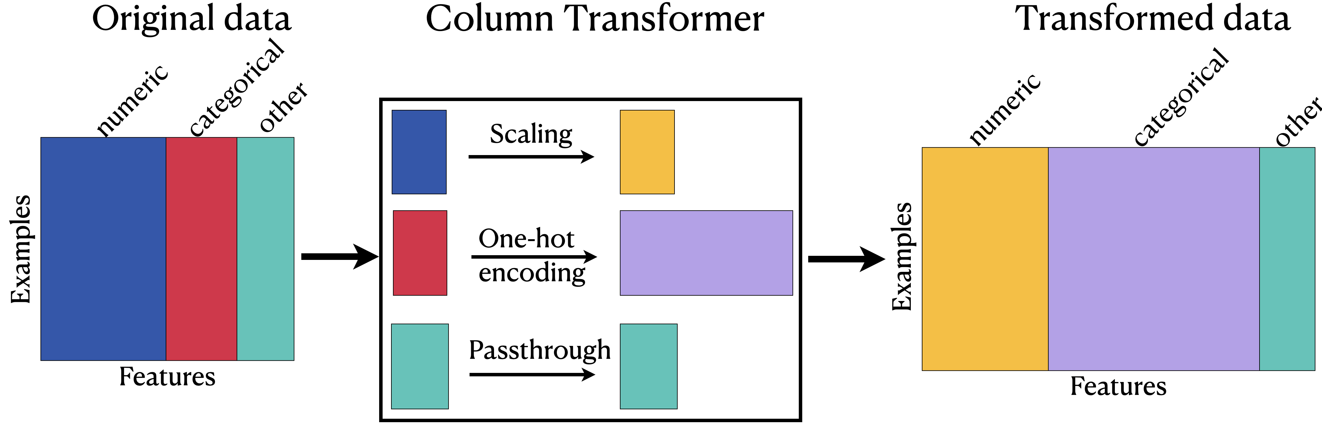
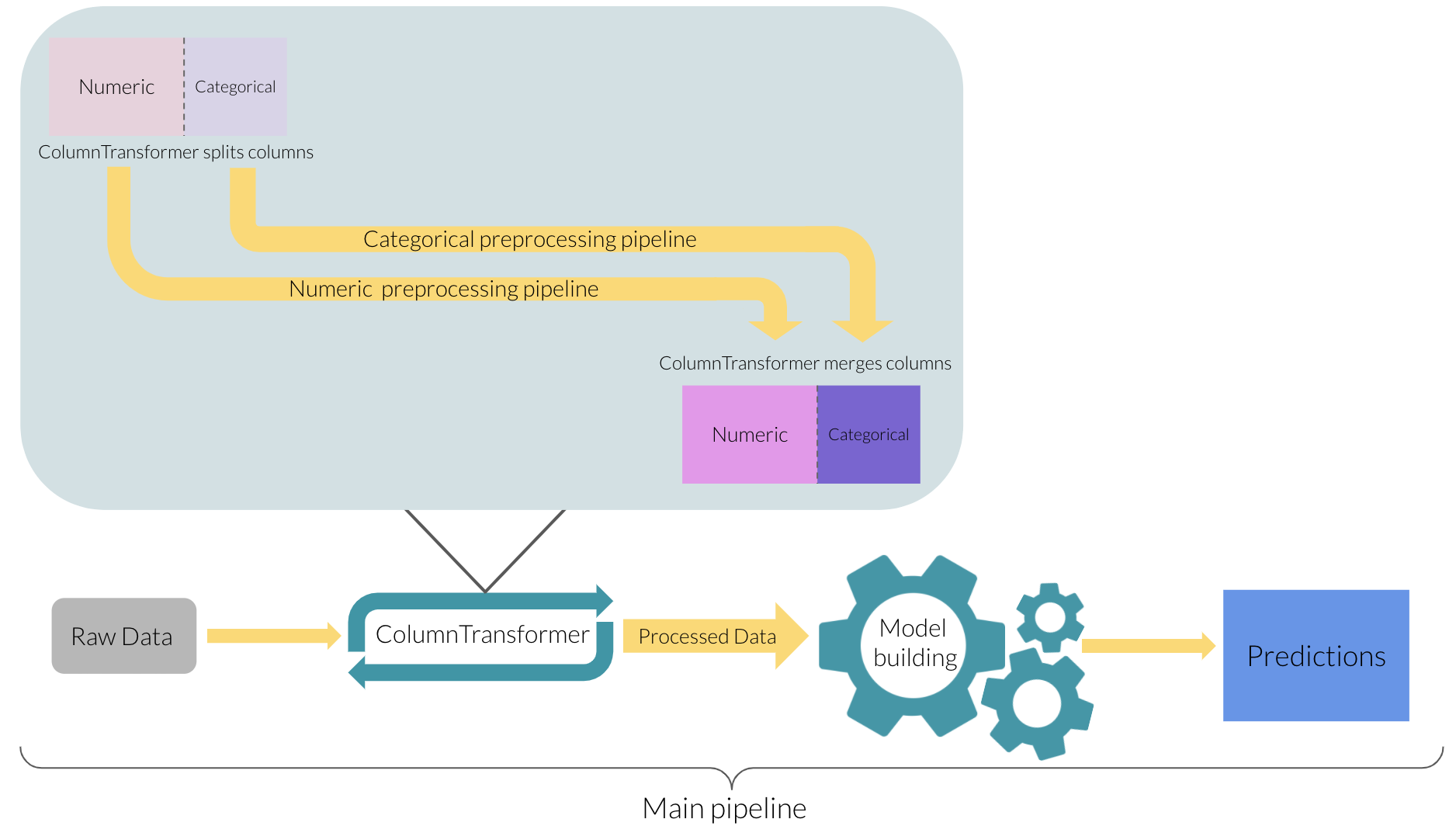
We can also look at this image which shows the more generic version of what happens in ColumnTransformer and where it stands in our main pipeline.
5.9.1.1. Do we need to preprocess categorical values in the target column?#
Generally, there is no need for this when doing classification.
sklearnis fine with categorical labels (y-values) for classification problems.
5.10. Simplifying the Pipeline syntax#
When we looked at our California housing dataset we had the following pipelines, ColumnTransformer and main pipeline with our model.
# transform numeric features
numeric_transformer = Pipeline(
steps=[("imputer", SimpleImputer(strategy="median")),
("scaler", StandardScaler())]
)
# transform categorical features
categorical_transformer = Pipeline(
steps=[("imputer", SimpleImputer(strategy="constant", fill_value="missing")),
("onehot", OneHotEncoder(handle_unknown="ignore"))]
)
# combine both transformations
col_transformer = ColumnTransformer(
transformers=[
("numeric", numeric_transformer, numeric_features),
("categorical", categorical_transformer, categorical_features)
],
remainder='passthrough'
)
# combine column transformation with model
pipe = Pipeline(
steps=[
("preprocessor", col_transformer),
("reg", KNeighborsRegressor())])
pipe
Pipeline(steps=[('preprocessor',
                 ColumnTransformer(remainder='passthrough',
                                   transformers=[('numeric',
                                                  Pipeline(steps=[('imputer',
                                                                   SimpleImputer(strategy='median')),
                                                                  ('scaler',
                                                                   StandardScaler())]),
                                                  Index(['longitude', 'latitude', 'housing_median_age', 'households',
       'median_income', 'rooms_per_household', 'bedrooms_per_household',
       'population_per_household'],
      dtype='object')),
                                                 ('categorical',
                                                  Pipeline(steps=[('imputer',
                                                                   SimpleImputer(fill_value='missing',
                                                                                 strategy='constant')),
                                                                  ('onehot',
                                                                   OneHotEncoder(handle_unknown='ignore'))]),
                                                  Index(['ocean_proximity'], dtype='object'))])),
('reg', KNeighborsRegressor())])In a Jupyter environment, please rerun this cell to show the HTML representation or trust the notebook. On GitHub, the HTML representation is unable to render, please try loading this page with nbviewer.org.
Pipeline(steps=[('preprocessor',
ColumnTransformer(remainder='passthrough',
                  transformers=[('numeric',
                                 Pipeline(steps=[('imputer',
                                                  SimpleImputer(strategy='median')),
                                                 ('scaler', StandardScaler())]),
                                 Index(['longitude', 'latitude', 'housing_median_age', 'households',
       'median_income', 'rooms_per_household', 'bedrooms_per_household',
       'population_per_household'],
      dtype='object')),
                                ('categorical',
                                 Pipeline(steps=[('imputer',
                                                  SimpleImputer(fill_value='missing',
                                                                strategy='constant')),
                                                 ('onehot',
                                                  OneHotEncoder(handle_unknown='ignore'))]),
Index(['ocean_proximity'], dtype='object'))])),
('reg', KNeighborsRegressor())])ColumnTransformer(remainder='passthrough',
transformers=[('numeric',
Pipeline(steps=[('imputer',
SimpleImputer(strategy='median')),
('scaler', StandardScaler())]),
Index(['longitude', 'latitude', 'housing_median_age', 'households',
       'median_income', 'rooms_per_household', 'bedrooms_per_household',
       'population_per_household'],
dtype='object')),
('categorical',
Pipeline(steps=[('imputer',
SimpleImputer(fill_value='missing',
strategy='constant')),
('onehot',
OneHotEncoder(handle_unknown='ignore'))]),
Index(['ocean_proximity'], dtype='object'))])Index(['longitude', 'latitude', 'housing_median_age', 'households',
'median_income', 'rooms_per_household', 'bedrooms_per_household',
'population_per_household'],
dtype='object')SimpleImputer(strategy='median')
StandardScaler()
Index(['ocean_proximity'], dtype='object')
SimpleImputer(fill_value='missing', strategy='constant')
OneHotEncoder(handle_unknown='ignore')
passthrough
KNeighborsRegressor()
This is great but it seems quite a lot of typing.
Especially the naming of the different steps appears quite redundant.
Luckily there are methods that help make our life easier.
They are called make_pipeline and make_column_transformer
and creates automatic names for the pipeline steps.
from sklearn.pipeline import make_pipeline
from sklearn.compose import make_column_transformer
numeric_transformer = make_pipeline(
SimpleImputer(strategy="median"),
StandardScaler()
)
categorical_transformer = make_pipeline(
SimpleImputer(strategy="constant", fill_value="missing"),
OneHotEncoder()
)
col_transformer = make_column_transformer(
(numeric_transformer, numeric_features),
(categorical_transformer, categorical_features),
remainder='passthrough'
)
pipe = make_pipeline(col_transformer, KNeighborsRegressor())
pipe
Pipeline(steps=[('columntransformer',
ColumnTransformer(remainder='passthrough',
transformers=[('pipeline-1',
Pipeline(steps=[('simpleimputer',
SimpleImputer(strategy='median')),
('standardscaler',
StandardScaler())]),
Index(['longitude', 'latitude', 'housing_median_age', 'households',
       'median_income', 'rooms_per_household', 'bedrooms_per_household',
       'population_per_household'],
dtype='object')),
('pipeline-2',
Pipeline(steps=[('simpleimputer',
SimpleImputer(fill_value='missing',
strategy='constant')),
('onehotencoder',
OneHotEncoder())]),
Index(['ocean_proximity'], dtype='object'))])),
('kneighborsregressor', KNeighborsRegressor())])In a Jupyter environment, please rerun this cell to show the HTML representation or trust the notebook. On GitHub, the HTML representation is unable to render, please try loading this page with nbviewer.org.
Pipeline(steps=[('columntransformer',
                 ColumnTransformer(remainder='passthrough',
                                   transformers=[('pipeline-1',
                                                  Pipeline(steps=[('simpleimputer',
                                                                   SimpleImputer(strategy='median')),
                                                                  ('standardscaler',
                                                                   StandardScaler())]),
                                                  Index(['longitude', 'latitude', 'housing_median_age', 'households',
       'median_income', 'rooms_per_household', 'bedrooms_per_household',
       'population_per_household'],
      dtype='object')),
                                                 ('pipeline-2',
                                                  Pipeline(steps=[('simpleimputer',
                                                                   SimpleImputer(fill_value='missing',
                                                                                 strategy='constant')),
                                                                  ('onehotencoder',
                                                                   OneHotEncoder())]),
                                                  Index(['ocean_proximity'], dtype='object'))])),
('kneighborsregressor', KNeighborsRegressor())])ColumnTransformer(remainder='passthrough',
transformers=[('pipeline-1',
Pipeline(steps=[('simpleimputer',
SimpleImputer(strategy='median')),
('standardscaler',
StandardScaler())]),
Index(['longitude', 'latitude', 'housing_median_age', 'households',
       'median_income', 'rooms_per_household', 'bedrooms_per_household',
       'population_per_household'],
dtype='object')),
('pipeline-2',
Pipeline(steps=[('simpleimputer',
SimpleImputer(fill_value='missing',
strategy='constant')),
('onehotencoder',
OneHotEncoder())]),
Index(['ocean_proximity'], dtype='object'))])Index(['longitude', 'latitude', 'housing_median_age', 'households',
'median_income', 'rooms_per_household', 'bedrooms_per_household',
'population_per_household'],
dtype='object')SimpleImputer(strategy='median')
StandardScaler()
Index(['ocean_proximity'], dtype='object')
SimpleImputer(fill_value='missing', strategy='constant')
OneHotEncoder()
passthrough
KNeighborsRegressor()
You can see that we get the same steps as above, but with generic names instead of the manually chosen ones.
5.11. Let’s Practice#
Refer to this dataframe to answer the following question and the textual representation of its corresponding pipeline to answer these questions.
       colour   location    shape   water_content  weight
0       red      canada      NaN         84          100
1     yellow     mexico     long         75          120
2     orange     spain       NaN         90          NaN
3    magenta     china      round        NaN         600
4     purple    austria      NaN         80          115
5     purple    turkey      oval         78          340
6     green     mexico      oval         83          NaN
7      blue     canada      round        73          535
8     brown     china        NaN         NaN        1743
9     yellow    mexico      oval         83          265
Pipeline(
    steps=[('columntransformer',
               ColumnTransformer(
                  transformers=[('pipeline-1',
                                  Pipeline(
                                    steps=[('simpleimputer',
                                             SimpleImputer(strategy='median')),
                                           ('standardscaler',
                                             StandardScaler())]),
                      ['water_content', 'weight', 'carbs']),
                                ('pipeline-2',
                                  Pipeline(
                                    steps=[('simpleimputer',
                                             SimpleImputer(fill_value='missing',
                                                                strategy='constant')),
                                           ('onehotencoder',
                                             OneHotEncoder(handle_unknown='ignore'))]),
                      ['colour', 'location', 'seed', 'shape', 'sweetness',
                                                   'tropical'])])),
         ('decisiontreeclassifier', DecisionTreeClassifier())])
1. How many categorical columns are there and how many numeric?
2. What preprocessing step is being done to both numeric and categorical columns?
3. How many columns are being transformed in pipeline-1?
4. Which pipeline is transforming the categorical columns?
5. What model is the pipeline fitting on?
True or False
6. If there are missing values in both numeric and categorical columns, we can specify this in a single step in the main pipeline.
7. If we do not specify remainder="passthrough" as an argument in ColumnTransformer, the columns not being transformed will be dropped.
8. Pipeline() is the same as make_pipeline() but make_pipeline() requires you to name the steps.
Solutions!
3 categoric columns and 2 numeric columns
Imputation
3
pipeline-2DecisionTreeClassifierFalse - You would specify different imputation strategies for numeric and categorical columns.
True - If you do not specify
remainder='passthrough'inColumnTransformer, the columns not explicitly specified in transformers will be dropped. By default,remainderis set to ‘drop’.False - Both
Pipeline()andmake_pipeline()create a pipeline, but they differ in how you specify and name the steps.Pipeline()requires you to provide a list of (name, transform) tuples, where the names are strings that you choose.make_pipeline()generates names automatically based on the types of the transformers. You don’t have to explicitly name the steps when usingmake_pipeline().
5.12. Text Data#
Machine Learning algorithms that we have seen so far prefer numeric and fixed-length input that looks like this.
and $\(y = \begin{bmatrix}spam \\ non spam \\ spam \end{bmatrix}\)$
But what if we are only given data in the form of raw text and associated labels? We will talk about this in more detail in next lecture, but let’s start with an introduction here.
How can we represent such data into a fixed number of features?
5.12.1. Spam/non-spam toy example#
Would you be able to apply the algorithms we have seen so far on the data that looks like this?
and
In categorical features or ordinal features, we have a fixed number of categories.
In text features such as above, each feature value (i.e., each text message) is going to be different.
How do we encode these features?
5.13. Bag of words (BOW) representation#
One way is to use a simple bag of words (BOW) representation which involves two components.
The vocabulary (all unique words in all documents)
A value indicating either the presence or absence or the count of each word in the document.
Grammatical rules and word order does not matter in a BOW representation, which might seem like an oversimplification but it can still be effective for ML purposes.
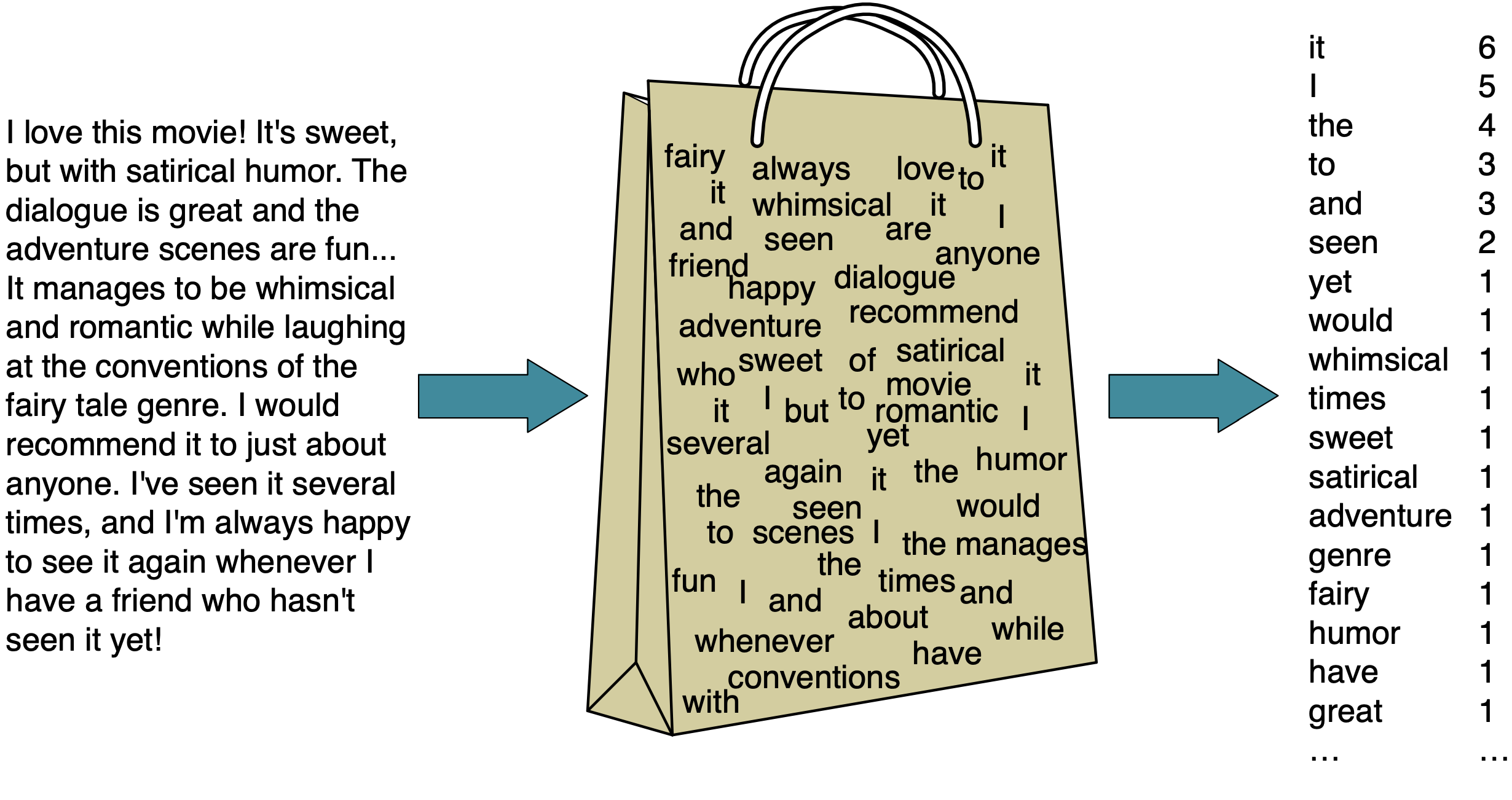
Attribution: Daniel Jurafsky & James H. Martin
5.13.1. Extracting BOW features using scikit-learn#
Let’s say we have 1 feature in our X dataframe consisting of the following text messages.
In our target column, we have the classification of each message as either spam or non spam.
X = [
    "URGENT!! As a valued network customer you have been selected to receive a £900 prize reward!",
    "Lol you are always so convincing.",
    "Nah I don't think he goes to usf, he lives around here though",
    "URGENT! You have won a 1 week FREE membership in our £100000 prize Jackpot!",
    "Had your mobile 11 months or more? U R entitled to Update to the latest colour mobiles with camera for Free! Call The Mobile Update Co FREE on 08002986030",
    "As per your request 'Melle Melle (Oru Minnaminunginte Nurungu Vettam)' has been set as your callertune for all Callers. Press *9 to copy your friends Callertune"]

y = ["spam", "non spam", "non spam", "spam", "spam", "non spam"]
We import a tool called CountVectorizer.
from sklearn.feature_extraction.text import CountVectorizer
We use CountVectorizer to convert text data into feature vectors where:
Each row represents a “document” (e.g., a text message in our example).
Each feature is a unique word in the text
Each feature value represents the frequency or presence/absence of the word in the given message
In the NLP community, a text data set is referred to as a corpus (plural: corpora).
The features should be a 1 dimension array as an input.
vec = CountVectorizer()
X_counts = vec.fit_transform(X);
bow_df = pd.DataFrame(X_counts.toarray(), columns=vec.get_feature_names_out(), index=X)
bow_df
| 08002986030 | 100000 | 11 | 900 | all | always | are | around | as | been | ... | update | urgent | usf | valued | vettam | week | with | won | you | your | |
|---|---|---|---|---|---|---|---|---|---|---|---|---|---|---|---|---|---|---|---|---|---|
| URGENT!! As a valued network customer you have been selected to receive a £900 prize reward! | 0 | 0 | 0 | 1 | 0 | 0 | 0 | 0 | 1 | 1 | ... | 0 | 1 | 0 | 1 | 0 | 0 | 0 | 0 | 1 | 0 |
| Lol you are always so convincing. | 0 | 0 | 0 | 0 | 0 | 1 | 1 | 0 | 0 | 0 | ... | 0 | 0 | 0 | 0 | 0 | 0 | 0 | 0 | 1 | 0 |
| Nah I don't think he goes to usf, he lives around here though | 0 | 0 | 0 | 0 | 0 | 0 | 0 | 1 | 0 | 0 | ... | 0 | 0 | 1 | 0 | 0 | 0 | 0 | 0 | 0 | 0 |
| URGENT! You have won a 1 week FREE membership in our £100000 prize Jackpot! | 0 | 1 | 0 | 0 | 0 | 0 | 0 | 0 | 0 | 0 | ... | 0 | 1 | 0 | 0 | 0 | 1 | 0 | 1 | 1 | 0 |
| Had your mobile 11 months or more? U R entitled to Update to the latest colour mobiles with camera for Free! Call The Mobile Update Co FREE on 08002986030 | 1 | 0 | 1 | 0 | 0 | 0 | 0 | 0 | 0 | 0 | ... | 2 | 0 | 0 | 0 | 0 | 0 | 1 | 0 | 0 | 1 |
| As per your request 'Melle Melle (Oru Minnaminunginte Nurungu Vettam)' has been set as your callertune for all Callers. Press *9 to copy your friends Callertune | 0 | 0 | 0 | 0 | 1 | 0 | 0 | 0 | 2 | 1 | ... | 0 | 0 | 0 | 0 | 1 | 0 | 0 | 0 | 0 | 3 |
6 rows × 72 columns
5.13.2. Important hyperparameters of CountVectorizer#
There are many useful and important hyperparameters of CountVectorizer.
binary:Whether to use absence/presence feature values or counts.
max_features:Only considers top
max_featuresordered by frequency in the corpus.
max_df:When building the vocabulary ignore terms that have a document frequency strictly higher than the given threshold.
min_df:When building the vocabulary ignore terms that have a document frequency strictly lower than the given threshold.
ngram_range:Consider word sequences in the given range.
X
['URGENT!! As a valued network customer you have been selected to receive a £900 prize reward!',
 'Lol you are always so convincing.',
 "Nah I don't think he goes to usf, he lives around here though",
 'URGENT! You have won a 1 week FREE membership in our £100000 prize Jackpot!',
 'Had your mobile 11 months or more? U R entitled to Update to the latest colour mobiles with camera for Free! Call The Mobile Update Co FREE on 08002986030',
 "As per your request 'Melle Melle (Oru Minnaminunginte Nurungu Vettam)' has been set as your callertune for all Callers. Press *9 to copy your friends Callertune"]
CountVectorizer is carrying out some preprocessing because of the default argument values.
Converting words to lowercase (
lowercase=True). Take a look at the word “urgent” In both cases.getting rid of punctuation and special characters (
token_pattern ='(?u)\\b\\w\\w+\\b')
We can use CountVectorizer() in a pipeline just like any other transformer.
from sklearn.svm import SVC

pipe = make_pipeline(CountVectorizer(), SVC())

pipe.fit(X, y)
Pipeline(steps=[('countvectorizer', CountVectorizer()), ('svc', SVC())])In a Jupyter environment, please rerun this cell to show the HTML representation or trust the notebook. On GitHub, the HTML representation is unable to render, please try loading this page with nbviewer.org.
Pipeline(steps=[('countvectorizer', CountVectorizer()), ('svc', SVC())])CountVectorizer()
SVC()
pipe.predict(X)
array(['spam', 'non spam', 'non spam', 'spam', 'spam', 'non spam'],
      dtype='<U8')
pipe.score(X, y)
1.0
Here we get a perfect score on our toy dataset data that it’s seen already.
How well does it do on unseen data?
X_new = [
    "Congratulations! You have been awarded $1000!",
    "Mom, can you pick me up from soccer practice?",
    "I'm trying to bake a cake and I forgot to put sugar in it smh. ",
    "URGENT: please pick up your car at 2pm from servicing",
    "Call 234950323 for a FREE consultation. It's your lucky day!" ]

y_new = ["spam", "non spam", "non spam", "non spam", "spam"]
pipe.score(X_new,y_new)
0.8
It’s not perfect but it seems to do well on this data too.
5.13.3. Is this a realistic representation of text data?#
Of course, this is not a great representation of language.
We are throwing out everything we know about language and losing a lot of information.
It assumes that there is no syntax and compositional meaning in language.
…But it works surprisingly well for many tasks and we will talk more about a classifier called Naive Bayes in next lecture, which uses this technique and was the state of the art classifier for detecting spam for a long time.
5.14. Let’s Practice#
1. What is the size of the vocabulary for the examples below?
X = [ "Take me to the river",
    "Drop me in the water",
    "Push me in the river",
    "Dip me in the water"]
2. Which of the following is not a hyperparameter of CountVectorizer()?
a) binary
b) max_features
c) vocab
d) ngram_range
3. What kind of simplified representation can we use for text data in ML?
True or False
4. As you increase the value for the max_features hyperparameter of CountVectorizer, the training score is likely to go up.
5. If we encounter a word in the validation or the test split that’s not available in the training data, we’ll get an error.
Solutions!
10
c)
vocabBag of Words
True
False
5.15. Let’s Practice - Coding#
We are going to bring in a new dataset for you to practice on. This dataset contains a text column containing tweets associated with disaster keywords and a target column denoting whether a tweet is about a real disaster (1) or not (0). This is available in your data folder, and the original source is here.
# Loading in the data
tweets_df = pd.read_csv('data/tweets_mod.csv').dropna(subset=['target'])

# Split the dataset into the feature table `X` and the target value `y`
X = tweets_df['text']
y = tweets_df['target']

# Split the dataset into X_train, X_test, y_train, y_test
X_train, X_test, y_train, y_test = train_test_split(X, y, test_size=0.2, random_state=7)

X_train
1684    It still hasn’t sunk in my LSU TIGAHS. Are Nat...
2650    Victims of the anomaly are kept in a quarantin...
3605    #StormBrendan Update-8.00 Tuesday.: Significan...
3458                   this storm is violent af. bathong.
2460    6 killed in China after massive EXPLODING sink...
                              ...
1603    IIIIII, I KEEP A RECORD OF THE WRECKAGE OF MY ...
2550    494. On account of the snowstorm, all the trai...
537     Israel moves to demolish the house belonging t...
1220    Sitting in the front room with my bride and th...
175     Which she eventually had to apologize for and ...
Name: text, Length: 3200, dtype: object
Make a pipeline with
CountVectorizeras the first step andSVC()as the second.Perform 5 fold cross-validation on your pipeline to evaluate the model performance (also return the training score). Convert the results into a dataframe for nicer display.
What are the mean training and validation scores?
Train your pipeline on the full training set.
Score the pipeline on the test set.
Solutions
1.
pipe = make_pipeline(
    CountVectorizer(),
    SVC()
)
2.
pd.DataFrame(cross_validate(pipe, X_train, y_train, return_train_score=True)).mean()
fit_time       0.697432
score_time     0.147431
test_score     0.798438
train_score    0.971875
dtype: float64
3.
pipe.fit(X_train, y_train)
Pipeline(steps=[('countvectorizer', CountVectorizer()), ('svc', SVC())])In a Jupyter environment, please rerun this cell to show the HTML representation or trust the notebook. On GitHub, the HTML representation is unable to render, please try loading this page with nbviewer.org.
Pipeline(steps=[('countvectorizer', CountVectorizer()), ('svc', SVC())])CountVectorizer()
SVC()
4.
pipe.score(X_test, y_test)
0.8125
5.16. What We’ve Learned Today#
How to process categorical features.
How to apply ordinal encoding vs one-hot encoding.
How to use
ColumnTransformer,make_pipelinemake_column_transformer.How to work with text data.
How to use
CountVectorizerto encode text data.What the different hyperparameters of
CountVectorizerare.